Chapter 3 A model with a mean (one sample t-test)
In this chapter, we will start our journey into the General Linear Model with the most basic example within the GLM: a model concerning a single Normal distribution, where we are interested in statements about the mean of that distribution. The resulting test is also known as the one-sample t-test. We will look at the Normal distribution in detail, and cover estimation of its parameters, before focusing on testing hypotheses about the mean. We will also introduce confidence intervals as an alternative, but mostly equivalent means to make inferences about parameters. We end the chapter by looking at the assumptions of the model, and what happens to the testing procedure if those assumptions are false.
3.1 Numeric judgement and anchoring
In 1906, Sir Francis Galton attended The West of England Fat Stock and Poultry Exhibition in Plymouth. One of the attractions at the fair was a contest to guess the weight of a “dressed” ox on display. The nearest guess to the actual weight of the ox would win a prize, and a total of 800 attendees participated for a small fee. Not only was Francis Galton a eugenicist5 – and rightly condemned for this in more modern times – he was also a statistician, and bought the used tickets off the stall holder. Back home he analysed the 787 usable tickets and later published his findings (Galton, 1907). What surprised Galton was that while the individual guesses were often far from the true weight of the ox, the average guess of the group as a whole was highly accurate. Such findings are now often referred to as the “Wisdom of the crowds”.
Although the wisdom of the crowds has been demonstrated in various domains, from decades of research, we also know that human judgement is subject to a long list of biases. One such bias is called “anchoring”, and it pertains to the influence of prior exposure to a more or less arbitrary numerical value on the subsequent numerical judgement. For instance, if I ask you “How tall do you think Mount Everest is?”, but first state that Mount Everest is taller than 2000 feet, you are likely to give a smaller number than if I first state that Mount Everest is shorter than 45,500 feet.
In this example, we will focus on data obtained from a large scale replication study, covering the above described anchoring manipulation, as well as many other experiments (Klein et al., 2014). This “Many Labs” study contained data collected by a large number of labs from different countries, and here we will use data collected by Konrad Bocian and Natalia Frankowska from the University of Social Sciences and Humanities Campus in Sopot, Poland. In particular, we will focus on the judged height of Mount Everest (in meters, as their participants were Polish) after a low anchor (610 meters6). From the wisdom of the crowds idea, we might expect the average judgement to be identical (or at least very close) to the true height of Mount Everest, which is 8848 meters above sea level. On the other hand, if the low anchor biased the judgements, we might expect the average judgement to deviate from the true height.
3.1.1 Exploring the data
Before diving into statistical modelling, as discussed, it is always good to explore the data. There were judgements by \(n=109\) people in this dataset. A graphical overview in the form of a histogram and raincloud plot is given in Figure 3.1. The minimum judged height was 650 meters (so quite close to the anchor), and the maximum was 12,459 meters. The median judgement was 8000 and the mean 6312.193. The sample variance of the judgements was 9,742,645 and the sample standard deviation 3121.321.


Figure 3.1: Histogram and boxplot of participants’ judgments
Looking at Figure 3.1, you can see a peak in the distribution around the true height of Mount Everest (8848 meters), but the judgements are also quite varying, with a large number of judgements substantially below the actual height. This may be due to some people knowing the correct answer, whilst others don’t and have to guess. Those guessing would likely be more influenced by the low anchor. The question is whether, on average, the group’s judgements are equal to the actual height of Mount Everest.
3.2 A statistical model of judgements
Clearly, not everyone gave a correct answer, and there is substantial variation in people’s judgements. The goal of a statistical model is to account for this variation. In this chapter, we will consider one of the simplest statistical models for metric data such as the judgements, namely the Normal distribution. In this model, we will assume that the variation in judgements is entirely random. We may also assume that, on average, the judgements are equal to the actual height of Mount Everest, but some people will overestimate, and some people underestimate the height in their judgements. Moreover, we might assume that the probability of an underestimation is equal to the probability of an overestimation, and that very large over- or underestimations are less likely than smaller over- or underestimations. The Normal distribution encapsulates such assumptions.
3.2.1 The Normal distribution
The Normal distribution is the well-known bell-shaped curve depicted in Figure 3.2.

Figure 3.2: The Normal density function for \(\mu = 0\) and \(\sigma = 1\)
The curve is given by the following function:
\[\begin{equation} p(y) = \frac{1}{\sqrt{2 \pi} \sigma} e^{-\frac{(y-\mu)^2}{2\sigma^2}} \tag{3.1} \end{equation}\]
If that looks complicated, don’t worry. First, let me point out that \(\pi\) refers to the mathematical constant pi, i.e. \(\pi= 3.141593\ldots\), and \(e\) refers to the mathematical constant also known as Euler’s number, i.e. \(e = 2.718282\ldots\). They are known constants and not parameters. The Normal distribution does have two parameters: \(\mu\) (“mu”), the mean, and \(\sigma\) (“sigma”), also called the standard deviation. Confusingly, the formula above is not actually the formula for the Normal probability distribution. Rather, it is the formula of the Normal density function. The Normal distribution applies to continuous variables. Technically, you can’t assign a probability to a particular value of a continuous variable, you can only assign probabilities to ranges of values. This is because a continuous variable has an infinite number of values (even if we restrict ourselves to a range). If we gave each unique value a probability of anything larger than 0, the total probability would not be 1, but infinite. If you add up an infinite amount of values, no matter how tiny they are, at some point you would reach a sum of 1, and then you’d have to keep on adding more. No matter how large the sum becomes, you would have to keep on going. Adding up an infinite number of values is not light work…
While we can’t define probability of any particular value, the probability that an observation is within a particular range is well-defined. So, rather than asking “What is the probability that the height is exactly 8567.46384634748763…?”, we can ask “What is the probability that the height is between 8567 and 8568?”, or “What is the probability that the height is between 8567.575 and 8567.576?”. These probabilities are defined by the “area under the curve” within that range. Using calculus, they can be computed as:
\[p(a \leq Y \leq b) = \int_a^b \frac{1}{\sqrt{2 \pi} \sigma} e^{-\frac{(y-\mu)^2}{2\sigma^2}} d y\]
If you are unfamiliar with calculus and have never seen an integration sign (\(\int\)), don’t worry, you don’t have to solve equations like this, and there won’t be many more like this. You can just see it as a mathematical way of referring to the area under the curve between point \(a\) and \(b\). A proper probability density function respects the rule of total probability. The Normal distribution is defined over all real numbers (i.e. all possible numbers between minus infinity and infinity). Thus, the rule of total probability rquires that \(p(-\infty \leq Y \leq \infty) = 1\), and this is true for the Normal distribution. Figure 3.3 shows the probability of three ranges, each symmetrical around the mean. The probability of a value falling in the range between \(\mu - 3 \times \sigma\) and \(\mu + 3 \times \sigma\) is very close to 1. Hence, values more than three standard deviations from the mean are extremely unlikely.

Figure 3.3: Normal distribution and the probability of a value falling in one of three overlapping ranges. Note that the ranges are overlapping, so that the range between \(\mu - 3 \sigma\) and \(\mu + 3 \sigma\) also covers the range between \(\mu - 2 \sigma\) and \(\mu + 2 \sigma\), but that this isn’t shown in the colours.
Because the Normal distribution is symmetric, with a single peak in the middle at \(\mu\), the parameter \(\mu\) not only equals the mean, but also the median (50% of all values are lower than \(\mu\), and 50% are higher), and the mode.
The Normal distribution is rather popular in statistical modelling. One important reason we’ll mention later (which is the Central Limit Theorem). Here, we’ll focus on two properties that make the Normal distribution quite convenient to work with. Before we continue, let’s introduce some new notation. As before, we will use \(Y\) to denote the dependent variable (i.e. people’s judgements of the height of Mount Everest), and \(Y_i\) to denote the \(i\)-th value of the dependent variable (i.e. the judgement by participant \(i\)), where \(i=1,\ldots,n\). We will state the assumption that \(Y\) follows a Normal distribution as \[Y_i \sim \mathbf{Normal}(\mu,\sigma)\] You can read this as “\(Y_i\) is sampled from a Normal distribution with mean \(\mu\) and standard deviation \(\sigma\)”. So the tilde (\(\sim\)) stands for “sampled from”. When we denote distributions, such as the Normal distribution, we will use a bold font for the name of the distribution, and between the parentheses that follow we will indicate the parameters of the distribution.
3.2.2 Two useful properties of the Normal distribution
1. A linear transformation of a Normal-distributed variable is also Normal-distributed. More formally, if \[Y \sim \mathbf{Normal}(\mu_y, \sigma_y)\] and \[Y' = a + b \times Y\] i.e. a new variable \(Y'\) is constructed by multiplying \(Y\) by \(b\) and then adding a constant \(a\), the distribution of this new variable \(Y'\) is \[Y' \sim \mathbf{Normal}\left(a + b \times \mu_y, | b | \times \sigma_y\right)\] i.e. a Normal distribution with mean equal to the linear transformation of the mean of \(Y\), and standard deviation equal to the standard deviation of \(Y\) multiplied by the absolute value of \(b\).
For example, suppose a fast-food chain is known for its “mega-megalicious” burger. The weight of each handmade patty is Normal-distributed with a mean of 1.2 pounds, and a standard deviation of 0.16 pounds. We can work out the distribution of the weight in kilograms by first noting that 1 kilogram = 2.2046 pounds and conversely, that one pound is \(1/2.2046 = 0.4536\) kilograms. Weight in kilograms is thus a linear transformation of weight in pounds: \[\text{kg} = 0 + 0.4536 \times \text{lbs}\] with \(a=0\) and \(b=0.4536\). The distribution of the weight in kilograms is then a Normal distribution with mean \(0 + 0.4536 \times 1.2 = 0.5443\) kilograms, and standard deviation \(|0.4536| \times .16 = 0.0725\) kilograms.
As another example, we can standardize a Normal variable by subtracting the mean and then dividing by the standard deviation. The resulting variable is conventionally denoted as \[\begin{equation} Z = \frac{Y-\mu}{\sigma} \tag{3.2} \end{equation}\] and the transformation of \(Y\) to \(Z\) is also called the Z-transformation. We can view \(Z\) as a linear transformation of \(Y\) with \(a=-\frac{\mu_y}{\sigma_y}\) and \(b = \frac{1}{\sigma_y}\). So \(Z\) has a mean of \(\mu_z = -\frac{\mu_y}{\sigma_y} + \frac{1}{\sigma_y} \times \mu_y= 0\) and a standard deviation of \(\sigma_z = |\frac{1}{\sigma_y}|\sigma_y = 1\). A Normal-distribution with a mean of 0 and a standard deviation of 1 is also called a standard Normal distribution.
2. The sum of two Normal-distributed variables is also Normal-distributed. More formally, if \[Y_1 \sim \mathbf{Normal}(\mu_1,\sigma_1)\] and \[Y_2 \sim \mathbf{Normal}(\mu_2,\sigma_2)\] and \(Y_s\) is the sum of \(Y_1\) and \(Y_2\), i.e. \[Y_s = Y_1 + Y_2\], then \(Y_s\) is distributed as \[Y_s \sim \mathbf{Normal}\left(\mu_1 + \mu_2, \sqrt{\sigma_1^2 + \sigma^2_2}\right)\] i.e. a Normal distribution with mean equal to the sum of the mean of \(Y_1\) and the mean of \(Y_2\), and standard deviation equal to the square-root of the sum of the variance of \(Y_1\) and the variance of \(Y_2\).
As we will see, these properties will come in handy later. For instance, when working out the sampling distribution of the mean.
3.2.3 Back to anchoring
If people’s judgements are on average correct, this implies that \(\mu = 8848\). Alternatively, the average judgement might be biased, for instance because of the low anchor. If this is so, what would the average judgement be? It is difficult to make a clear prediction about this. If we can’t really come up with anything sensible, we may as well assume that this parameter can have any value, as we did for Paul’s probability of a correct prediction if he were (somewhat) psychic. We can then formulate our two alternative models for people’s judgements as:
- MODEL R: \(\quad Y_i \sim \mathbf{Normal}(8848, \sigma)\)
- MODEL G: \(\quad Y_i \sim \mathbf{Normal}(\mu, \sigma)\)
MODEL R is the restricted model, a special case of the more general MODEL G. The restriction is on \(\mu\). In MODEL G, the mean can take any value, so \(-\infty \leq \mu \leq \infty\) (remember that \(\infty\) stands for infinity). MODEL R picks a specific value \(\underline{\mu}\) from this infinite range, namely \(\mu = \overline{\mu} = 8848\). In both models, the standard deviation is not specified, so is considered unknown. Standard deviations, like variances, can never be negative, so at least we know that \(\sigma \geq 0\), but this is all that we will specify in advance for that parameter.
3.3 Parameter estimation
MODEL G has two parameters: the mean \(\mu\) and the standard deviation \(\sigma\). The maximum likelihood estimate of \(\mu\) is the sample mean:
\[\begin{equation} \hat{\mu} = \overline{Y} = \frac{\sum_{i=1}^n Y_i}{n} \tag{3.3} \end{equation}\]
The maximum likelihood estimate of the variance is the sample variance (see Equation (1.2)), i.e. \(\hat{\sigma}^2_\text{ML} = S^2\). However, this estimator of the variance is biased. It is therefore common to estimate the variance with the unbiased estimator: \[\begin{equation} \hat{\sigma}^2 = \frac{\sum_{i=1}^n (Y_i - \overline{Y})^2}{n-1} \tag{3.4} \end{equation}\] The difference is to divide the sum of squared deviations by \(n-1\), rather than by \(n\). Intuitively, you can think of the reason for this as follows: When we use the sample mean \(\overline{Y}\) rather than the true mean \(\mu\) in computing the variance, we don’t take into account that the sample mean is a noisy estimate of the true mean \(\mu\). Compared to \(\overline{Y}\), the true mean could be somewhat higher or lower, and therefore the sample variance is likely to be an underestimate of the true variance. In other words, it is biased. By dividing by \(n-1\) instead of \(n\), the resulting estimate is a little higher. It so happens this completely removes the bias. When \(n\) is large (i.e. there are a large number of observations), there will be little difference between the unbiased estimate and the sample variance, but for small \(n\) the difference will be more marked.
Note that the estimator above is for the variance \(\sigma^2\) (sigma squared, i.e. sigma raised to the power of 2), not for the standard deviation \(\sigma\). If we want an estimator of the standard deviation, we can simply take the square-root to get the following estimator of \(\sigma\):
\[\hat{\sigma} = \sqrt{\hat{\sigma}^2}\]
If the mean is known to equal a particular value, \(\mu = \underline{\mu}\), as in MODEL R, then we should use that value \(\underline{\mu}\) instead of \(\overline{Y}\) to estimate the variance and standard deviation. The unbiased estimate of the standard deviation for MODEL R is \[\hat{\sigma}_R = \sqrt{\frac{\sum_{i=1}^n (Y_i - \underline{\mu})^2}{n}}\] Perhaps confusingly, we can now divide by \(n\) instead of by \(n-1\) to get an unbiased estimate. The reason for this is that when we know the true mean, there is no estimation error like we had for \(\overline{Y}\), and hence no additional source of variability which would bias the estimate.
3.3.1 Sampling distribution of the estimated mean
Remember that the estimator of the mean is an algorithm that provides estimates from data. Different datasets will give different estimates, even though all these datasets are generated from the same Data Generating Process. Our model of the Data Generating Process is the Normal distribution, which has two parameters: \(\mu\) and \(\sigma\). Let’s pick some values for these parameters, so that we can use our model to simulate data. For instance, suppose the judgements are on average equal to the true value, so \(\mu = 8848\). Individual judgements are quite variable, however, so let’s take \(\sigma = 2000\). Figure 3.4 shows the distribution of the estimated mean of 10,000 data sets each consisting of \(n=109\) observations (the same number of observations as our anchoring data). Also shown (as a dotted line) is the Normal distribution of the model we used to generate the data. Clearly, the estimated means are much less variable than the simulated judgements themselves.

Figure 3.4: Estimated means for 10000 simulated data sets of \(n = 109\), drawn from a Normal distribution with mean 8848 and standard deviation 2000. The dotted line represents the Normal distribution from which the data sets were generated, and the solid line the theoretical distribution of the estimated means.
Simulating data and then looking at the resulting distribution of estimates is straightforward, but also noisy. Luckily, it is quite easy to derive the true distribution of the estimated means (i.e. the sample means). Using the two properties of the Normal distribution, we know that the sum of two Normal-distributed variables also follows a Normal distribution. This is easily generalized to the sum of any number of Normal-distributed variables. For instance, we can construct the distribution of the sum of three variables by adding the sum of two Normal-distributed variables (which we know is a Normal-distributed variable) to a third Normal-distributed variable: \(Y_s = (Y_1 + Y_2) + Y_3\). Hence, the sum of three Normal-distributed variables is also Normal-distributed. We can then take the sum of three variables, and add a fourth one, and this sum will also be Normal-distributed: \(Y_s = ((Y_1 + Y_2) + Y_3) + Y_4\), and so will the sum of five, six, and any number of Normal-distributed variables. This is a nice example of a recursive function.
In short, if each \(Y_i \sim \mathbf{Normal}(\mu,\sigma)\), then \[\sum_{i=1}^n Y_i \sim \mathbf{Normal}(n \mu, \sqrt{n}\sigma)\] Moreover, as we discussed earlier, we can view the mean as a linear transformation of this sum with \(a = 0\) and \(b=\frac{1}{n}\), from which we can derive that \[\overline{Y} \sim \mathbf{Normal}\left(\mu, \frac{\sigma}{\sqrt{n}}\right)\] Hence, the sampling distribution of the estimated means is a Normal distribution with a mean equal to \(\mu\). The estimator is thus unbiased. The standard deviation of the sampling distribution of the estimated means is equal to \(\frac{\sigma}{\sqrt{n}}\), i.e. the standard deviation of the dependent variable divided by \(\sqrt{n}\). The standard deviation of the sampling distribution of estimates is also called the standard error of the estimates. Dividing by \(\sqrt{n}\) implies that the standard deviation of the sample means is smaller than the standard deviation of the dependent variable. And, as \(n\) increases, it becomes smaller and smaller. The estimator is therefore also consistent. And, as it turns out, the estimator is also efficient.
To simulate judgements, we had to pick an arbitrary value of \(\sigma\). But how can we simulate the data when \(\sigma\) is unknown? We could of course use the unbiased estimate \(\hat{\sigma}\). For MODEL R and the present data, that would be \(\hat{\sigma} = 4021.562\), which is obviously substantially larger than the value of 2000 we used before. If we’d use this value to simulate data sets and look at the distribution of the sample mean, we’d get a similar plot to the one of Figure 3.4, but with a larger standard deviation.
Suppose that MODEL R is true, that the Data Generating Process indeed results in a Normal distribution of people’s judgements with a mean \(\mu = 8848\) and a standard deviation \(\sigma\). If we knew the value of \(\sigma\), then we’d know everything there is to know about the distribution of the DGP. And knowing this, we’d know everything there is to know about the distribution of the sample means. But we don’t know \(\sigma\). While it makes sense to use an estimate of \(\sigma\), this estimate will be noisy. We shouldn’t just pretend that our estimate \(\hat{\sigma}\) is identical to the true \(\sigma\). The problem is that different values of \(\sigma\) lead to different sampling distributions of the mean. Key to working out the sampling distribution of the mean when \(\sigma\) is unknown is to also take into account the sampling distribution of the estimates of \(\sigma\). Roughly, the idea is that, for a given data set, we can work out how likely different values of \(\sigma\) are, and we can then derive the average of all the Normal distributions that follow from each possible value of \(\sigma\). The resulting distribution is not a Normal distribution. It was derived by William Sealy Gosset (1876–1937) in 1904. Gosset worked as Head Experimental Brewer for Guinness in Dublin, and the company had a rule forbidding their chemists to publish their findings (Zabell, 2008). Gosset was able to convince his boss that his mathematical work was of no practical use to competing brewers, and was allowed to publish them in Student (1908), but under a pseudonym to avoid his colleagues getting similar ideas. “Student” was the pseudonym chosen by the managing director of Guinness, and hence the distribution is now known as Student’s t-distribution.

Figure 3.5: (Understandardized) Student t-distribution which is the true sampling distribution of the mean under MODEL R with unknown \(\sigma\) (solid line) and the Normal distribution that would be the sampling distribution if it were known that \(\sigma = \hat{\sigma}\) (broken line). Note that these curves are drawn for the case of \(n=10\) observations, to make the differences between the distributions more marked. For \(n=109\), the t-distribution is almost identical to the Normal distribution.
You can see a comparison of the t-distribution and the Normal distribution in Figure 3.5. The main thing to notice is that the t-distribution is also bell-shaped and symmetric, but it is wider (has fatter tails) than the Normal distribution. The difference between the t-distribution and Normal distribution depends on the value of \(n-1\). When \(n>30\), the difference is, for most practical purposes, negligible.
3.4 Testing whether \(\mu\) has a specific value
Our main interest here is to assess whether it is reasonable to assume that, in the Data Generating Process, the average judgement equals the true height of Mount Everest. More bluntly, we simply want to know whether \(\mu = 8848\).
3.4.1 The classical way
Now we know what happens to the estimate \(\hat{\mu}\) of MODEL G when MODEL R is in fact true, we can use a similar logic as before to decide when \(\hat{\mu}\) is different enough from \(\underline{\mu}\) to reject MODEL R. To work this out, it is convenient to standardize the sample mean by subtracting the (supposed) true average, and dividing by the standard error of the sample mean: \[\begin{equation} t = \frac{\hat{\mu} - \underline{\mu}}{\hat{\sigma}/\sqrt{n}} = \frac{\overline{Y} - \underline{\mu}}{\hat{\sigma}/\sqrt{n}} \tag{3.5} \end{equation}\] where \[\hat{\sigma} = \sqrt{\frac{\sum_{i=1}^n (Y_i - \overline{Y})^2}{n-1}}\] is the unbiased estimator of \(\sigma\). We call the resulting standardized value the \(t\) statistic. It is much like the \(Z\)-transformation, but now we’re using an estimated \(\hat{\sigma}\) rather than a known value. The standardized \(t\) statistic follows a \(t\) distribution with \(n-1\) degrees of freedom, which reflects the amount of data we used to estimate \(\sigma\). What we showed in Figure 3.5 was an “unstandardized” t-distribution, which also has a location and scale parameter. By standardizing \(t\), we don’t need to worry about these. Generally, when someone mentions the t-distribution, they refer to the standardized version, which has a single parameter, the degrees of freedom (commonly denoted with the Greek symbol \(\nu\), pronounced as “nu”; I will just use “degrees of freedom”, or \(df\) though). Back in the times of Gosset, this was particularly important, as there was no access to modern computers to quickly work out the probabilities for different versions of unstandardized t-distributions. Statisticians had to rely on tables for a standard version of a distribution, which were painstakingly computed by hand. In fact, the term “computer” originally referred to a person performing mathematical calculations. Complex, long, and often rather tedious calculations were performed by teams of such computers.
I won’t bore you with the mathematical details of the t-distribution. As I already mentioned, it looks quite like a Normal distribution. When the degrees of freedom get larger, the distributions looks more and more like the standard Normal distribution. Because we know that if MODEL R is true, the \(t\) statistic follows a t-distribution with \(n-1\) degrees of freedom, we know all there is to know about the sampling distribution of \(t\). If \(t\) is far away from 0, that means that the estimate \(\hat{\mu}\) of MODEL G is far away from the assumed value \(\underline{\mu}\) in MODEL R, and hence we have reason to reject MODEL R. Following the logic of the null-hypothesis significance test, we will limit the number of wrong rejections of MODEL R by choosing critical values such that \[p(t \leq \text{lower critical value} | \text{MODEL R}) + p(t \geq \text{upper critical value} | \text{MODEL R}) = \alpha\] The resulting critical regions are depicted in Figure 3.6.

Figure 3.6: Critical regions for rejecting \(H_0\): \(\mu = 8848\) with \(\alpha = .05\)
So how about the judgements in the anchoring experiment? Is it reasonable to assume that \(\mu = 8848\)? Let’s perform the test and see. For MODEL G, our estimated mean is \(\hat{\mu} = 6312.193\), and the unbiased estimate of the standard deviation is \(\hat{\sigma} = 3135.738\). The \(t\) statistic is then \[t = \frac{6312.193 - 8848}{3135.738/\sqrt{109}} = -8.443\] For a significance level of \(\alpha = .05\), we can use the t-distribution with 108 degrees of freedom to work out the lower and upper critical value as -1.982 and 1.982. Clearly, the value of the \(t\)-statistic that we computed is far below the lower critical value, which means we reject the null hypothesis. The associated \(p\)-value with this two-sided test (we would reject \(H_0\) if we had very large negative, as well as very large positive values of the \(t\) statistic), is \(p(t \leq -8.443| \text{df} = 108) + p(t \geq 8.443| \text{df} = 108) = p(|t| \geq 8.443| \text{df} = 108) < .001\). So, in conclusion, the \(t\)-statistic is in the critical region for our chosen significance level of \(\alpha = .05\), which leads us to reject the null hypothesis. Equivalently, the \(p\)-value, the probability of obtaining a \(t\) statistic equal to or more extreme than the one we found, is smaller than our chosen significance level \(\alpha=.05\), so we reject the null hypothesis. In our anchoring data, the “wisdom of crowds” doesn’t seem to hold, because the average judgement does not equal the true height of Mount Everest.
3.4.2 The model comparison way
There is an equivalent way to perform the hypothesis test that \(\mu = \underline{\mu}\), by directly comparing two versions of our statistical model, one in which we assume we know the value of \(\mu\) to be \(\underline{\mu}\) (MODEL R), and one in which we don’t (MODEL G). As we did for Paul the Octopus, we then look at the likelihood ratio to see whether MODEL R is tenable. Note that in both models, the standard deviation is considered unknown and will have to be estimated.
The procedure is essentially the same as before. We find a way to calculate the likelihood ratio, and work out the distribution of the likelihood ratio values we would get for repetitions of an experiment assuming MODEL R is true. Using this distribution, we can then work out a critical value, such that the probability of obtaining a likelihood ratio value equal to or smaller than it is equal to a significance level \(\alpha\), i.e. , \(p(\text{likelihood ratio } \leq \text{critical value} | \text{MODEL R}) = \alpha\). The derivation of the likelihood ratio is a little more complicated than before though. Feel free to glance over the following, as the derivation is not that important. The paragraphs marked with a vertical line in the left margin are more advanced and can be skipped without too much consequence.
When all observations \(Y_i\), \(i=1, \ldots, n\) are independent draws from a Normal distribution, then we can use the product rule to work out the joint “probability” (density value really) of all observations. That is, we use Equation (3.1) to compute \(p(Y_i)\), the density value of each observation, and then multiply these together: \[ \begin{aligned} p(Y_1, Y_2, \ldots, Y_n) &= p(Y_1) \times p(Y_2) \times \ldots \times p(Y_n) \\ &= \prod_{i=1}^n \frac{1}{\sqrt{2 \pi} \sigma} e^{-\frac{(Y_i-\mu)^2}{2\sigma^2}} \\ &= \left( \frac{1}{\sqrt{2 \pi} \sigma} \right)^n e^{ \frac{n}{2\sigma^2} \sum_{i=1}^n (Y_i - \mu)^2} \end{aligned} \] The \(\prod\) sign on the second line is similar to the summation sign, but tells you to multiply all the values that follow it, so e.g. \[\prod_{i=1}^3 Y_i = Y_1 \times Y_2 \times Y_3\] On the third line, we make use of the fact that \(e^a \times e^b = e^{a + b}\). We can write the likelihood ratio of MODEL R over MODEL G as \[ \begin{aligned} L\!R(R,G) &= \frac{\left( \frac{1}{\sqrt{2 \pi} \hat{\sigma}_{ml,R}} \right)^n e^{ \frac{n}{2\hat{\sigma}^2_{ml,R}} \sum_{i=1}^n (Y_i - \mu)^2}}{\left( \frac{1}{\sqrt{2 \pi} \hat{\sigma}_{ml,G}} \right)^n e^{ \frac{n}{2\hat{\sigma}^2_{ml,G}} \sum_{i=1}^n (Y_i - \mu)^2}} \\ &= \frac{ \left(\sqrt{\frac{2\pi}{n} \sum_{i=1}^n(Y_i - \underline{\mu})^2}\right)^{-n} e^{\frac{\sum_{i=1}^n(Y_i - \underline{\mu})^2}{2 \sum_{i=1}^n(Y_i - \underline{\mu})^2/n}}}{\left(\sqrt{\frac{2\pi}{n} \sum_{i=1}^n(Y_i - \overline{Y})^2}\right)^{-n} e^{ \frac{\sum_{i=1}^n (Y_i - \overline{Y})^2}{2 \sum_{i=1}^n (Y_i - \overline{Y})^2/n}} } \\ &= \left(\frac{\sum_{i=1}^n(Y_i - \underline{\mu})^2}{\sum_{i=1}^n(Y_i - \overline{Y})^2}\right)^{-n/2} \end{aligned} \]
What is interesting to point out is that, on the last line of the equation above, we see that the two main ingredients of the likelihood ratio are sums of squared deviations. Moreover, as the deviations are between observations and the mean (either assumed mean or sample mean), these sums of squared deviations are very closely related to variances. As we will see later, “sums of squares” are important quantities when comparing General Linear Models.
While the likelihood ratio is reasonably straightforward to compute, it is not easy to derive the sampling distribution of the likelihood ratio. Previously, we could work out the distribution of the likelihood ratio when MODEL R is true relatively easily from the Binomial distribution of the outcomes. We can do something similar here, which effectively means transforming the likelihood ratio into a statistic we do know the distribution of, or conversely, transforming a statistic we know the distribution of into the likelihood ratio. To do this, first we can rewrite \[\sum_{i=1}^n(Y_i - \underline{\mu})^2 = \sum_{i=1}^n(Y_i - \overline{Y} + \overline{Y} - \underline{\mu})^2 = n(\overline{Y} - \underline{\mu})^2 + \sum_{i=1}^n(Y_i - \overline{Y})^2\] and filling this in the numerator of the likelihood ratio gives \[L\!R(R,G) = \left(1 + \frac{n(\overline{Y} - \underline{\mu})^2}{\sum_{i=1}^n(Y_i - \overline{Y})^2}\right)^{-n/2}\] For a given experiment or study, we can treat the number of observations \(n\) as a given fixed number. What we are really interested in is the part of the likelihood ratio that depends on the data. If we take the square root of this part, we get \[\frac{|\overline{Y} - \underline{\mu}|}{\sqrt{\sum_{i=1}^n(Y_i - \overline{Y})^2}} = \sqrt{n (n-1)} \times | t |\] with \(t\) defined as in Equation (3.5). When the absolute value of the \(t\) statistic becomes larger, the likelihood ratio value becomes smaller (less supportive of MODEL R). We can thus view the likelihood ratio as a (rather complicated) transformation of the absolute value of the \(t\) statistic. The distribution of the likelihood ratio is then also a (rather complicated) transformation of the distribution of the \(t\)-statistic. Just like the coin tossing model, where the likelihood ratio was effectively a transformation of the statistic \(k\) (the number of correct guesses), and the distribution of the likelihood ratio a transformation of the distribution of \(k\), i.e. the Binomial distribution.
What all this means is that the one-sample t-test, as worked out before, is equivalent to a likelihood ratio test comparing MODEL R to MODEL G. Whether you perform the test in the “classic” way by computing the \(t\) statistic and assessing the magnitude of this in the \(t\) distribution, or whether you compute a likelihood ratio and assess the magnitude of this in the distribution of the likelihood ratio under MODEL R, you will get exactly the same outcome.
3.5 Confidence intervals
Confidence intervals are interval estimates. That is, rather than providing a single point estimate of a parameter, they specify a range of values for a parameter. That range is chosen in a precise, but somewhat counter-intuitive and difficult to understand manner. Ideally, what you might want to obtain is a range such that you can be certain that, with a specified probability, the true parameter is within this range. Unfortunately, this is not what confidence intervals do. Like much of Frequentist statistics, confidence intervals concern “the long run”, they are based on the idea of an infinite number of possible (simulated) datasets from a true model. Confidence intervals are the result of an algorithm which is constructed in such a way that the ranges it produces will, for a specified proportion of all those possible datasets, contain the true value of the parameter.
While difficult to interpret properly, the confidence interval for the mean of Normal interval with unknown standard deviation is straightforward to compute: \[\begin{equation} \hat{\mu} \pm t_{n-1; 1- \frac{\alpha}{2}} \frac{\hat{\sigma}}{\sqrt{n}} \tag{3.6} \end{equation}\] where \(t_{n-1; 1- \frac{\alpha}{2}}\) stands for the upper critical value of a test with significance level \(\alpha\). In other words, we take our estimate of the mean (i.e. \(\hat{\mu} = \overline{Y}\)), and add or subtract from that a multiple of the estimated standard error of the mean (which is \(\frac{\hat{\sigma}}{\sqrt{n}}\); remember that the standard error of a statistic is the standard deviation of the sampling distribution of that statistic). The multiple is derived from the t-distribution. As explained earlier, for the Normal distribution, we know that 95% of the observations lie in the range between \(\mu - 1.96 \times \sigma\) and \(\mu + 1.96 \times \sigma\). Similarly, for the Normal distribution, 95% of the sample means lie in the range between \(\mu - 1.96 \times \frac{\sigma}{\sqrt{n}}\) and \(\mu + 1.96 \times \frac{\sigma}{\sqrt{n}}\). The value \(t_{n-1; \frac{\alpha}{2}}\) is effectively a replacement for 1.96, which takes into account that we have estimated \(\sigma\).
Figure 3.7: \(\text{95%}\) confidence intervals for 100 simulated datasets with \(\mu=8848\) and \(\sigma=2000\). Most of the intervals contain the true value \(\mu\), but some do not. If we would simulate an infinite number of datasets, then exactly \(\text{95%}\) of the intervals would contain \(\mu\), and exactly \(\text{5%}\) would not.
Earlier on, we simulated datasets of size \(n=109\) from a Normal distribution with mean \(\mu = 8848\) and \(\sigma = 2000\). In Figure 3.7 we show the resulting 95% confidence intervals (now estimating \(\sigma\) from the data) for 100 of such simulated datasets. As you can see, the location, and the width of each confidence interval is different. Moreover, you can see that while most of the confidence intervals contain the true value \(\mu = 8848\), some don’t. Indeed, 6 out of 100 confidence intervals do not include the true value of \(\mu\), which is pretty close to 5%.
For the judgements in the anchoring experiment, the estimated mean was \(\hat{\mu} = 6312.193\), the unbiased estimate of the standard deviation was \(\hat{\sigma} = 3135.738\), and the upper critical value was \(t_{108, .975} = 1.982\). Thus, the confidence interval is \[ \begin{aligned} \text{95% confidence interval} &= \hat{\mu} - t_{n-1; 1 - \frac{\alpha}{2}} \times \frac{\hat{\sigma}}{\sqrt{n}} \leq \mu \leq \hat{\mu} + t_{n-1; 1- \frac{\alpha}{2}} \times \frac{\hat{\sigma}}{\sqrt{n}} \\ &= 6312.193 - 1.982 \times \frac{3135.738}{\sqrt{109}} \leq \mu \leq 6312.193 + 1.982 \times \frac{3135.738}{\sqrt{109}} \\ &= 5716.848 \leq \mu \leq 6907.537 \end{aligned} \]
Confidence intervals can be used to perform null hypothesis significance tests. In fact, a confidence interval contains all values of \(\underline{\mu}\) for which MODEL R would not be rejected with the current data. In other words, if the confidence interval includes the value of \(\underline{\mu}\) of interest (i.e. \(\underline{\mu} = 8848\) in our example), that means that the null hypothesis would not be rejected. In addition, we can also determine a whole range of other values of \(\underline{\mu}\) which, if purported as a null hypothesis, would also not be rejected. In that sense, a confidence interval provides more information than a simple “reject” or “not reject” decision of a null hypothesis significance test. If a confidence interval is very wide, that implies the significance test has low power. Of course, what “very wide” is, depends on the scale of the data, and a subjective evaluation by the researcher.
There have been calls to abandon hypothesis tests in favour of estimation and reporting confidence intervals (e.g. Cumming, 2014). Given the tricky interpretation of confidence intervals (Richard D. Morey, Hoekstra, Rouder, Lee, & Wagenmakers, 2016), and their rather close ties to significance tests, such ideas seem to promise more than they can deliver. There is no need to abandon either significance tests or confidence intervals, provided you know how to interpret them.
3.6 Effect size
Whether an observed deviation between the sample mean \(\overline{Y}\) and assumed mean \(\underline{\mu}\) is significant, depends on the power of the test. The power of a test, as you may recall, is the probability of a test statistic exceeding the critical value(s) when the null hypothesis is false (i.e., when the true mean \(\mu\) does not equal the assumed mean \(\underline{\mu}\)). This, in turn, depends to a large part on the number of observations (\(n\)). If you look closely at the definition of the \(t\)-statistic (Equation (3.5)), you might see that, for any given values of \(\overline{Y}\), \(\underline{\mu}\), and \(S\), the value of \(t\) increases with \(n\). This is because the more observations we have, the more precisely we can estimate the true mean \(\mu\) from the sample mean \(\overline{Y}\). So that’s all good. But as a consequence, if we have enough data, even the tiniest deviation between \(\overline{Y}\) and \(\underline{\mu}\) would give a significant test result. Whilst that is “all good” statistically speaking, in practical terms, we might not be all that interested in such small deviations from theoretical predictions. In addition to considering significance, it is useful to consider the size of the effect we have observed. By “effect”, we simply mean the deviation between the sample mean and assumed mean. As this deviation is dependent on the scale of measurement, it is useful to standardize the deviation in some way. A common way to standardize effect sizes is to make them relative to the variability in the data, in the same way as is done in \(Z\) scores. This provides us with what is commonly known as Cohen’s \(d\): \[\begin{equation} \text{Cohen's } d = \frac{\overline{Y} - \underline{\mu}}{\hat{\sigma}} \tag{3.7} \end{equation}\] For our anchoring example, Cohen’s \(d\) is \[d = \frac{6312.193 - 8848}{3135.738} = -0.809\]
Cohen’s \(d\) quantifies an effect in units of the standard deviation in the sample data. As a rule of thumb, an absolute value of \(|d| = 0.2\) is considered a small effect, an absolute value of \(|d| = 0.5\) a medium effect, and an absolute value of \(|d| = 0.8\) a large effect (Cohen, 1988). Thus, the effect-size we found can be classified as large. These rule-of-thumb values, relative to the Normal distribution, are depicted in Figure 3.8. As you can see, even “large” effect sizes are still quite close to the center of the distribution. For example, 21.19% of observations from the Data Generating Process would exceed the deviation specified as a large positive effect size. But you should keep in mind that the objective of an effect size here is to quantify the deviation between a sample mean and an assumed mean, not between observations and that assumed mean.

Figure 3.8: Small, medium, and large values of Cohen’s \(d\) in context of the data distribution.
Comparing Equation (3.7) to (3.5), we can see that these look almost the same. The only difference is that the \(t\) statistic divides the estimated standard deviation by \(\sqrt{n}\), as this provides the standard error of the mean. For a one-sample t-test, Cohen’s \(d\) can then also be computed as \(t/\sqrt{n}\). This shows that, to an extent, Cohen’s \(d\) removes the effect of \(n\) from the \(t\) statistic, and is not “inflated” as sample size increases. In addition to providing test results, it is generally a good idea to also provide the effect size as additional information.
3.7 Assumptions
When we started modelling the data, we assumed each judgement was effectively an independent random draw from a Normal distribution. In MODEL R, we assumed that the mean of that Normal distribution was \(\mu = 8848\), while in MODEL G, we left both the mean and the standard deviation unknown. Both models thus assume the judgements follow a Normal distribution. Looking at Figure 3.1, you might wonder whether that’s a reasonable assumption. The histogram doesn’t look exactly Normal. With real and limited data, histograms can be deceiving though. A Q-Q (quantile-quantile) plot aims to provide a better means to visually inspect whether data (approximately) follows an assumed distribution. Quantiles are cut points dividing the range of a probability distribution into continuous intervals with equal probabilities, or dividing the observations in a sample in the same way. Percentiles are an example of quantiles, which divide a probability distribution into ranges each containing .01 of the total probability (i.e. 1%). By ordering the values of a variable in a data set in increasing order of magnitude, you can also obtain “empirical quantiles”. Suppose you have 5 observations ordered in increasing magnitude:
1, 4, 4.5, 9, 20
For each value, you can determine the proportion of values in the data which are equal or smaller than it. For instance, the proportion of observations equal to or smaller than 1 is \(1/5 = 0.2\), the proportion of observations equal to or smaller than 4 is \(2/5 = 0.4\), the proportion of observations equal to or smaller than 4.5 is \(3/5 = 0.6\), etc. For each of these proportions, we can also work out the corresponding value of the variable for the probability of a value equal to smaller than it equals this proportion. For instance, for a Normal distribution with mean \(\mu=7\) and standard deviation \(\sigma = 7\), the quantile such that \(p(\text{value } \leq \text{ quantile}) = .2\) is 1.109, and the quantile such that \(p(\text{value } \leq \text{ quantile}) = .4\) is 5.227. In a Q-Q plot, the values of the observed data are plotted against these theoretical quantiles in a scatter-plot. If the data follows the assumed distribution, the empirical quantiles should generally match the theoretical quantiles, and hence the points in the plot should roughly lie on a straight line. Figure 3.9 shows such a Q-Q plot for the judgements. As you can see, rather than on a straight-line, the points seem to lie on an s-shaped curve, which indicates that the assumption of a Normal distribution might not be a good match to the data.

Figure 3.9: A Quantile-Quantile plot for the judgments of the height of Mount Everest
There are also two common tests for the null hypothesis that the distribution is Normal: the Kolmogorov-Smirnov, and the Shapiro-Wilk test. The former is a generic test, which can be used to check for other distributions besides the Normal one as well. The second one only focuses on the Normal distribution, and because it was specifically designed for this distribution, it is more powerful. I’m not going to describe how these tests actually work. You can look that up elsewhere if you like. I will tell you that both tests reject the null-hypothesis of a Normal distribution. For both tests, the \(p\)-value (the probability of obtaining a test result equal to or more extreme, given that the null hypothesis of a Normal distribution is true), is \(p<.001\). I should also caution you in relying too much on such tests. If you have large datasets, the tests are rather powerful, and may therefore reject the null hypothesis of a Normal distribution when there is just a small deviation from Normality in the data. Such small deviations might be rather inconsequential, so you should use your judgement and also rely on visual inspection of histograms and Q-Q plots. For the current data, both the plots and the tests indicate quite some deviation from a Normal distribution…
Perhaps there are really two groups of participants: those who know the height of the Mount Everest, and those who don’t. The first group will provide a highly accurate answer (allowing for small deviations, as their knowledge may not be exact), while the second group will guess, providing much more variable judgements which are more likely to be influenced by the anchor. If the judgements of each of these groups can be represented by a Normal distribution, but with different means and variances, then the distribution as a whole might look a bit like the one depicted in Figure 3.10. This is also called a mixture distribution and clearly, it is not a Normal distribution. How bad would it be if this were there case?

Figure 3.10: A bimodal distribution, arising when there are two groups of participants: those with good knowledge who provide answers close to the true height of Mount Everest, and those with poor knowledge, providing much more variable judgements. The distribution for each group is depicted by dotted lines, and the distribution over both groups as a solid line.
This is where things get a bit messy. One thing to realise is that we are mainly interested in the mean judgement, and whether this equals 8848 meters. We needed to make an assumption about the distribution of the judgements to (1) determine an appropriate estimator of the mean, and (2) derive a sampling distribution of the estimated means. In making inferences about the true mean of the judgements, we only really need to focus on this sampling distribution. And as it happens, an important result in statistics tells us that, no matter what distribution the data itself follows, if we use enough observations, the sampling distribution of the mean will be very close to Normal. This result is called the Central Limit Theorem.
3.8 The Central Limit Theorem
A main reason that the Normal distribution is used so often (and perhaps called “Normal”, rather than “Abnormal”), is due to a mathematical fact known as the Central Limit Theorem:
Definition 3.1 (Central Limit Theorem) The distribution of the sum of \(n\) independent variables approaches the Normal distribution as the number of variables approaches infinity (\(n \rightarrow \infty\)).
This is quite an amazing theorem. Although you might wonder why you should care about sums of an infinite number of random variables, there are two things to note. Firstly, the rate at which the distribution “approaches” the normal distribution can be rather fast. Secondly, as we showed when we discussed two useful properties of the Normal distribution, the sample mean can be viewed as a normalized sum of \(n\) variables: \(\overline{Y} = \frac{1}{n} \sum_{i=1}^n Y_i\). So the Central Limit Theorem applies also to the sample mean, and implies that as long as the size of the samples is large enough, the sample mean will follow a Normal distribution.
3.8.1 The Central Limit Theorem in action
To see the central limit theorem in action, let’s pick an arbitrary probability distribution over 5 values, as shown in Figure 3.11. This will be the true distribution (i.e. the Data Generating Process) from which we can draw or simulate values.

Figure 3.11: An aribitrary probability distribution over 5 values, clearly not a Normal distribution!
When we repeatedly draw 5 values and calculate the mean over these 5 observations, we can look at the distribution of these sampled means. This is shown in Figure 3.12. You can see that even when we draw just 5 values from a decidedly non-Normal distribution, the sample distribution of the resulting average already has the characteristic bell-shaped curve.
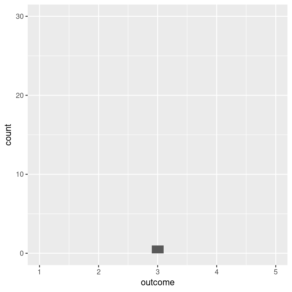
Figure 3.12: The distribution of the mean of 5 observations by simulating 200 data sets (from the distribution in Figure 3.11)
From the Central Limit Theorem, we can conclude that if we focus on the mean of a sufficiently large number of independent observations, we can reasonably assume that the sampling distribution of the mean will be a Normal distribution, even when the distribution from which the actual values were drawn is far from Normal. We can also use this to argue that the \(t\)-statistic is a valid means to test our hypothesis even when the data is not Normal-distributed. Indeed, simulations show that hypothesis tests with the \(t\)-statistic are valid for sufficiently large data sets even when the distribution of the observations is far from Normal (e.g. Lumley, Diehr, Emerson, & Chen, 2002).
Finally, the Central Limit Theorem may also be applied to justify the assumption of a Normal distribution, at least for certain variables. For instance, in (cognitive) psychology, we might imagine that processes such as perception and judgement rely on processing and transforming information, and that various processing and transformation steps are subject to many independent sources of noise (e.g., things we might call visual, neural, and memory noise). If these sources of noise combine additively, we could argue that the resulting percept or judgement will follow a Normal distribution.
3.8.2 Bootstrapping a statistic
The crucial thing to realise is that the assumption that the data is Normal-distributed is used to derive the sampling distribution of the test statistic. The sampling distribution of the test statistic allows us to calculate a \(p\)-value, and if the true sampling distribution of the statistic is different from what is assumed, then the \(p\)-value will be wrong. If the data is Normal-distributed, then we are guaranteed that the sampling distribution of the \(t\) statistic follows a t-distribution. If the data is not Normal-distributed, the sampling distribution of the \(t\) statistic may still be indistinguishable from a t distribution. In that case, the \(p\)-value would still be highly accurate, and we would not need to worry that the data is not Normal-distributed. In short, what we really want to know is whether the assumed distribution of a test statistic is approximately correct.
This is not something we can know for sure. All we have is a sample from the Data Generating Process; we do not know the true distribution of the data. But we can use this sample to do something similar as I did above to show the Central Limit Theorem in action: we can repeatedly draw samples and check the resulting distribution. In this case, we will treat the sample as what can be termed an empirical distribution. We can draw, with replacement, a large number of samples of size \(n\) from the data, and then check the distribution of the sample mean, or even better, the distribution of the \(t\) statistic. We need to draw samples with replacement (which means that the same observation can occur multiple times in our generated samples) to ensure that we obtain different generated samples. This procedure is also called a nonparametric bootstrap (Davison & Hinkley, 1997). It can be useful for a variety of purposes, including the computation of robust confidence intervals and hypothesis testing. Here, we use it to assess whether the assumed distribution by a parametric test such as the \(t\)-test seems reasonable.
Figure 3.13 shows the distribution of the sample mean and the \(t\)-statistic for a total of 100,0000 bootstrap samples, drawn with replacement from the empirical distribution of the data (Figure 3.1). As these plots indicate, whilst the empirical distribution looks far from Normal, the sampling distribution of the mean does not appear to deviate too far from a Normal distribution. Whilst not perfect, both the histogram and Q-Q plot show that the distribution is approximately Normal. The sampling distribution of the \(t\) statistic matches the assumed t distribution somewhat less well, with signs of left-skew. As such, the results of the \(t\)-test may be somewhat biased. This would be of particular concern when the observed effect was small and the test result close to the border of significance. Given the large magnitude of the \(t\)-statistic we computed for the actual data, and the very low \(p\)-value, it doesn’t seem likely that these are due to wrongly assuming a t distribution.
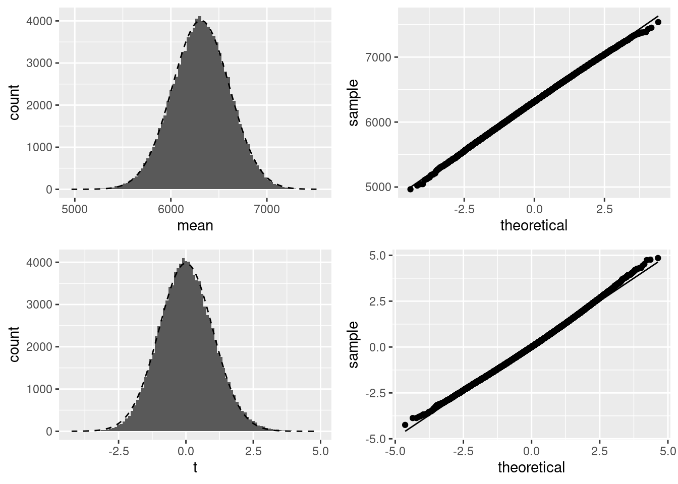
Figure 3.13: Boostrapped sample means and \(t\) statistics, using 100,000 bootstrap samples from the empirical distribution. For both the sample mean and \(t\) statistic, we show a histogram with the assumed theoretical distribution overlaid, and a Q-Q plot.
3.9 In practice
The one-sample t-test is perhaps one of the simplest statistical hypothesis tests. Simplicity is not a bad thing. If you can formulate a hypothesis in terms of an exact value of the true mean should take, that is a sign of an advanced science. Unfortunately, such precise predictions are rare in psychology. But in those occasions where you can use a one-sample t-test, here is some practical advice on how to proceed:
- Explore the data. In particular, check for outliers, which in this case are observations very far removed from the sample mean. Remember that in a Normal distribution, values which are more than 3 standard deviations removed from the mean are very rare. Whilst not impossible, such rare observations can severely bias the estimated mean. For example, if one participant in the anchoring experiment would have estimated the height of Mount Everest as one million meters, the sample mean would change rather dramatically. Consequently, the result of a statistical test could be entirely due to a single observation, effectively rendering all other observations in the data meaningless. In such cases, there is good reason to remove these unduly influential observations from the data. But this should always be done with caution. We will discuss outliers in more detail in Section 5.9.
- After removing outliers if necessary, assess whether the assumptions underlying the test are reasonable. This is, in my opinion, best done graphically. Plot the distribution of the variable of interest with e.g. a histogram, raincloud and Q-Q plot. Inspect these carefully. What you are looking for is relatively large deviations from a Normal distribution.
- Conduct the analysis and report the results. When reporting the results, make sure that you include all relevant statistics. For example, one way to write the results of anchoring analysis is as follows:
To assess bias in participant’s judgements of the height of Mount Everest, we conducted a one-sample \(t\)-test, against the null hypothesis that the average judgement equals the true height of Mount Everest (i.e. 8848 meters). In our sample of \(n=109\) participants, the average judgement was \(M = 6,312.19\), 95% CI \([5,716.85, 6,907.54]\). This is a significant difference from the null hypothesis of \(\mu = 8848\), \(t(108) = -8.44\), \(p < .001\), with an effect size of Cohen’s \(d = -0.809\), which can be considered large.