Chapter 10 Repeated-measures ANOVA
In this chapter, we will discuss how to deal with the non-independence of errors that can result from repeated measures of the same individual or from other groupings in the data, within the context of ANOVA-type analyses (i.e. a GLM with only categorical predictors). The resulting class of models is known as repeated-measures ANOVA. We will consider one way to construct this class of models, by constructing new dependent variables by applying orthogonal contrasts to create difference scores between the observed dependent variables. For each of these new dependent variables, we can use a GLM as usual. The main conceptual leap will be in interpreting these new dependent variables, which we’ll call within-subjects composite scores. The alternative approach is to apply contrast codes to the different “units of observation” (e.g. participants), and then treat this as a factorial design involving a mix of fixed and random experimental factors. As random and fixed effects are more straightforwardly dealt with in mixed-effects regression models – the topic of the next chapter – we will leave such considerations until later. The way we’ll will discuss repeated-measures ANOVA is close to how most modern computational approaches actually conduct these analyses.
10.1 Non-independence in linear models
The General Linear Model we have considered thus far can be stated as follows:
\[Y_i = \beta_0 + \beta_1 \times X_{1,i} + \beta_2 \times X_{2,i} + \ldots + \beta_m \times X_{m,i} + \epsilon_i \quad \quad \quad \epsilon_i \sim \mathbf{Normal}(0,\sigma_\epsilon)\] The assumptions of this model concern the errors, or residuals, \(\epsilon_i\). These are assumed to be independent and identically distributed (iid), following a Normal distribution with a mean of 0 and a standard deviation \(\sigma_\epsilon\).
You can expect violations of the iid assumption if data are collected from “units of observation” that are clustered in groups. A common example of this in psychology is when you repeatedly observe behaviour from the same person.23 For example, suppose participants in an experiment perform two tests to measure their working memory capacity. A person with a high working memory capacity would likely score high on both tests, whilst a person with a low working memory capacity would likely score low on both. In that case, the scores in the two tests are correlated and hence not independent. If the model does not adequately account for this, then the errors (residuals) would also not be independent. Violating the independence or errors assumption implies that the General Linear Model is misspecified, and does not account for all the structure in the data. This has consequences for the tests of parameters of the model. In addition to the test statistics no following the assumed distributions, the tests often have less power than when properly accounting for the dependencies. Following Charles M. Judd et al. (2011), the approach we take here is to remove the dependencies by transforming the data. In a nutshell, using orthogonal contrast codes, we transform a set of correlated dependent variables (e.g. two tests of working memory) into a set of orthogonal (uncorrelated) dependent variables. We then apply General Linear Models to each of these transformed dependent variables.
10.2 The cheerleader effect
The attractiveness of a person’s face is traditionally considered to be related to physical features, such as how symmetrical the features are, how close a face is to the “average” face over many people, and sexual dimorphism (whether a face looks exclusively male or female). However, there is also evidence that perceived facial attractiveness can vary due to factors outside of the face. In what has become known as the “cheerleader effect”, the same face is perceived to be more attractive when seen in a group, as compared to when it is seen alone. Walker & Vul (2014) proposed that the cheerleader effect arises due to people encoding faces in a hierarchical manner. When presented with a group of faces, people encode the display by first calculating an average face for the group, and then encoding individual faces as deviations from the group average. Because faces which are closer to the average face tend to be perceived as more attractive than individual faces, the encoded group average lifts the attractiveness of each face in the group, resulting in each face in the group being perceived as more attractive than if it were presented by itself.
Carragher, Thomas, Gwinn, & Nicholls (2019) set out to test this explanation. In one part of their study (Experiment 1), they let participants rate the attractiveness of a face when presented by itself (the Alone condition), as part of a group of different faces (the Different condition), or as part of a group of similar faces (the Similar condition). There were two variants of the latter condition, and participants encountered only one of them in the experiment. In the Identical condition, the group consisted of three copies of exactly the same photo. In the Variant condition, the group consisted of three different photos of the same face.24 The authors argued that if the hierarchical-encoding explanation for the cheerleader effect is true, then the cheerleader effect should not be observed in the Identical condition. This is because the average of three identical photos is just the photo itself, so there should be no difference between an encoded average face and the face itself. In the Variant condition however, variability between the different photos of the same face might still lead to an average face which is deemed more attractive than each individual face.
The design of the study is an example of a 2 (Version: Identical, Variant) by 3 (Presentation: Alone, Different, or Similar) design. The first factor (Version) varied between people, and the second (Presentation) within people (each participant rated a face in each of the three conditions). The rated attractiveness of the faces in the different conditions are provided in Figure 10.1.

Figure 10.1: Attractiveness ratings for photo’s of faces when presented alone, as part of a group of dissimilar faces (Different), or as part of a group of similar faces (Similar), which are either identical (Identical) or different photos (Variant) of the same face.
10.3 As a oneway ANOVA
To keep matters relatively simple, we will for now just consider the \(n=31\) participants in the Variant conditions. We can now treat the study as a oneway design, with three levels (Presentation: Alone, Different, or Similar) that all vary within-participants. As the cheerleader effect predicts that faces presented as part of a group will be rated as more attractive, and that this effect will be larger if there is more variety in the faces within the group, a reasonable set of contrast codes is:
| \(c_1\) | \(c_2\) | |
|---|---|---|
| Alone | \(-\tfrac{2}{3}\) | \(0\) |
| Different | \(\tfrac{1}{3}\) | \(\tfrac{1}{2}\) |
| Similar | \(\tfrac{1}{3}\) | \(-\tfrac{1}{2}\) |
The first contrast code reflects the expectation that a face in a group (Different or Similar) will be rated as more attractive than faces in the Alone condition. The second contrast reflects the expectation that a face surrounded by different faces will be rated as more attractive than when surrounded by more similar faces.
If we were to (wrongly!) treat all ratings as independent, and analyse the data with a regular oneway ANOVA, we would obtain the results in Table 10.1. As you can see, this analysis indicates there is no effect of presenting a face alone or in a group.
| \(\hat{\beta}\) | \(\text{SS}\) | \(\text{df}\) | \(F\) | \(p(\geq \lvert F \rvert)\) | |
|---|---|---|---|---|---|
| Intercept | 47.43 | 209177 | 1 | 2062.61 | 0.000 |
| Presentation | 36 | 2 | 0.18 | 0.840 | |
| \(\quad X_1\) (D+S vs A) | 1.30 | 35 | 1 | 0.34 | 0.559 |
| \(\quad X_2\) (D vs S) | -0.19 | 1 | 1 | 0.01 | 0.941 |
| Error | 9127 | 90 |
The problem with this analysis is that it ignores the (on occasion rather large) differences between participants in how attractive they find a face on average (i.e. over the three conditions). Table 10.2 shows the attractiveness ratings for 10 participants in the Variant condition. You can see there that when a participant rates a face as relatively attractive when presented alone, (s)he also tends to rate the face as relatively attractive when shown in a group of faces. Some participants (e.g. participant 37) rate the face as relatively unattractive in all conditions. This indicates individual differences in how attractive people find a face. Simply put: people’s tastes differ. Whilst that may be interesting in its own right, for the purposes of the experiment, we do not care about such individual differences. What we want to know is whether the attractiveness of a face increases when presented as part of a group vs when presented in isolation. To answer this question, we can’t completely ignore individual differences.
| Participant | Alone | Different | Similar | Average | D-A | S-A |
|---|---|---|---|---|---|---|
| 36 | 56.32 | 55.92 | 54.30 | 55.5 | -0.40 | -2.02 |
| 37 | 13.31 | 13.52 | 11.64 | 12.8 | 0.21 | -1.67 |
| 39 | 49.81 | 49.77 | 51.20 | 50.3 | -0.03 | 1.40 |
| 40 | 47.10 | 52.48 | 53.19 | 50.9 | 5.38 | 6.09 |
| 41 | 38.93 | 41.62 | 42.13 | 40.9 | 2.69 | 3.20 |
| 42 | 60.04 | 58.93 | 59.47 | 59.5 | -1.11 | -0.57 |
| 44 | 44.74 | 47.02 | 50.47 | 47.4 | 2.28 | 5.73 |
| 45 | 45.24 | 43.92 | 46.22 | 45.1 | -1.32 | 0.98 |
| 46 | 36.79 | 37.28 | 35.80 | 36.6 | 0.49 | -0.99 |
| 47 | 53.78 | 52.69 | 52.90 | 53.1 | -1.08 | -0.88 |
10.4 Oneway repeated-measures ANOVA
For each participant, we could consider whether the rating in e.g. the Different condition is higher than the rating in the Alone condition. These difference scores are provided in the D-A and S-A columns in Table 10.2. For participant 36, the rating in the Different condition is a little lower than their rating in the Alone condition, and for participant 37, it is a little higher. These difference scores remove variability in how attracted people are to a face in general. The difference scores just reflect whether people find a face more or less attractive when presented in the context of a group of faces, compared to when presented alone. We can then simply ask whether these differences are, on average, positive (indicating increased attractiveness) or negative (indicating decreased attractiveness). We can answer this question by using a one-sample t-test on the difference scores, comparing a general intercept-only MODEL G to an even simpler MODEL R where we fix the intercept to 0. If we can reject the null hypothesis that the mean of the difference is equal to 0, that is evidence of an effect of the experimental manipulation.
For example, we can compare attractiveness ratings between the Different and Alone conditions by, for the D-A difference scores, comparing a MODEL G \[\begin{aligned} (\text{D - A})_i &= Y_{i,\text{D}} - Y_{i,\text{A}} \\ &= \beta_0 + \epsilon_{\text{D-A},i} \end{aligned}\] to a MODEL R: \[\begin{aligned} (\text{D - A})_i &= Y_{i,\text{D}} - Y_{i,\text{A}} \\ &= 0 + \epsilon_{\text{D-A},i} \end{aligned}\]
This comparison is a test whether the mean of the D-A difference score is equal to 0. The result of this test is \(F(1,30) = 10.52\), \(p= .003\). We can therefore conclude there is evidence for a difference between the Different and Alone presentions, as would be expected from the “cheerleader effect”.
Using a similar model comparison approach for the S-A difference scores, we obtain a test result of \(F(1,30) = 10.28\), \(p= .003\). So, if we focus on differences between the conditions “within persons” (by computing differences between the conditions for each person), we find evidence that both the Different and Similar condition differ from the Alone condition. On average, participants’ rating of the attractiveness of a face was 1.21 points higher when presented amongst a group of different faces, and 1.4 points higher when presented amongst a group of similar faces, compared to when the face was presented by itself. Given that attractiveness was rated on a scale between 1-100, these are not large differences, but they are statistically significant.
10.4.1 Within-subjects composite scores
The idea of computing difference scores and then using these in linear models is essentially how we will test for effects of manipulations that vary within persons. To do this more generally, we will apply orthogonal contrast codes to compute such difference scores. We will refer to the resulting within-person-difference-scores as within-subjects composite scores.
We will use the same contrast codes as before, but denote them as \(d_j\) to separate them from between-subjects contrasts (\(c_j\)):
| \(d_1\) | \(d_2\) | |
|---|---|---|
| Alone | \(-\tfrac{2}{3}\) | \(0\) |
| Different | \(\tfrac{1}{3}\) | \(\tfrac{1}{2}\) |
| Similar | \(\tfrac{1}{3}\) | \(-\tfrac{1}{2}\) |
For each within-subjects contrast \(d_j\), we compute a within-subjects composite score as: \[\begin{equation} W_{j,i} = \frac{\sum_{k=1}^g d_{j,k} Y_{i,k}}{\sqrt{\sum_{k=1}^g d_{j,k}^2}} \tag{10.1} \end{equation}\] The top part of this equation (the numerator) is just the sum of a participant \(i\)’s score in each condition \(k\) multiplied by the corresponding value of contrast code \(d_j\). The bottom part (the denominator) is a scaling factor, computed as the square-root of the sum of the squared contrast values. The reason for applying this scaling factor is to make the sums of squares of the resulting analyses add up to the total sum of squares (i.e. the Sum of Squared Error of an intercept-only model). Otherwise, it is not of theoretical importance.
As an example, let’s compute the within-subjects composite scores for participant 36 in Table 10.2. For contrast \(d_1\), we compute \[\begin{aligned} W_{1,36} &= \frac{-\tfrac{2}{3} \times 56.32 + \tfrac{1}{3} \times 55.92 + \tfrac{1}{3} \times 54.30}{\sqrt{ \left(-\tfrac{2}{3}\right)^2 + \left(\tfrac{1}{3}\right)^2 + \left(\tfrac{1}{3}\right)^2)}} \\ &= \frac{-0.81}{\sqrt{\tfrac{6}{9}}} = -0.99 \end{aligned}\] For contrast \(d_2\), the within-subjects composite is computed as: \[\begin{aligned} W_{2,36} &= \frac{\tfrac{1}{2} \times 55.92 + (-\tfrac{1}{2}) \times 54.30}{\sqrt{\left(\tfrac{1}{2}\right)^2 + \left(-\tfrac{1}{2}\right)^2)}} \\ &= \frac{-0.81}{\sqrt{\tfrac{2}{4}}} = 1.15 \end{aligned}\] Table 10.3 shows the resulting values for other participants as well.
| Participant | Alone | Different | Similar | \(W_0\) | \(W_1\) | \(W_2\) |
|---|---|---|---|---|---|---|
| 36 | 56.32 | 55.92 | 54.30 | 96.2 | -0.99 | 1.15 |
| 37 | 13.31 | 13.52 | 11.64 | 22.2 | -0.60 | 1.33 |
| 39 | 49.81 | 49.77 | 51.20 | 87.1 | 0.56 | -1.01 |
| 40 | 47.10 | 52.48 | 53.19 | 88.2 | 4.68 | -0.50 |
| 41 | 38.93 | 41.62 | 42.13 | 70.8 | 2.40 | -0.36 |
| 42 | 60.04 | 58.93 | 59.47 | 103.0 | -0.69 | -0.38 |
| 44 | 44.74 | 47.02 | 50.47 | 82.1 | 3.27 | -2.44 |
| 45 | 45.24 | 43.92 | 46.22 | 78.2 | -0.14 | -1.63 |
| 46 | 36.79 | 37.28 | 35.80 | 63.4 | -0.20 | 1.05 |
| 47 | 53.78 | 52.69 | 52.90 | 92.0 | -0.80 | -0.15 |
The first within-subjects composite variable (\(W_1\)) reflects the difference between the average of the Different and Similar conditions and the Alone condition. If the mean of this composite variable is positive, that indicates that faces in the Different and Similar condition are on average rated as more attractive than in the Alone condition. If the mean of this composite variable is negative, that indicates that faces in the Different and Similar condition are on average rated as less attractive than in the Alone condition. If the mean is equal to 0, that indicates there is no difference in attractiveness ratings between the marginal mean of the Different and Similar conditions, compared to the Alone condition. To test whether this latter option is truem we can compare a MODEL G \[W_{1,i} = \beta_0 + \epsilon_i\] to a MODEL R: \[W_{1,i} = 0 + \epsilon_i\] The Sum of Squared Error of MODEL R is \(\text{SSE}(R) = 123.28\), and for MODEL G this is \(\text{SSE}(G) = 88.33\). There are \(n=31\) participants, and \(\text{npar}(R) = 0\) and \(\text{npar}(G) = 1\). The test result of the model comparison is therefore \(F(1,30) = 11.87\), \(p= .002\). We can thus reject the null hypothesis that there is no difference between the Alone condition and the marginal mean of the other two conditions. The estimated intercept of MODEL G is \(\hat{\beta}_0 = 1.06\). Due to the scaling applied in the within-subjects composite, this intercept does not equal the average of \(\frac{Y_{i,D} + Y_{i,S}}{2} - Y_{i,A}\). To get this value, we need to rescale the within-subjects composite to the scale of the dependent variable. We do this by dividing the estimated parameter by the scaling factor. The scaling factor equals \(\sqrt{ \left(-\tfrac{2}{3}\right)^2 + \left(\tfrac{1}{3}\right)^2 + \left(\tfrac{1}{3}\right)^2} = \sqrt{\tfrac{6}{9}}\). So \[\frac{\overline{Y}_{D} + \overline{Y}_{S}}{2} - \overline{Y}_{A} = \frac{1.06}{\sqrt{\tfrac{6}{9}}} = 1.3\] We can conduct a similar model comparison for the second within-subjects composite, \(W_2\). The Sum of Squared Error of MODEL R is \(\text{SSE}(R) = 40.17\), and for MODEL G this is \(\text{SSE}(G) = 39.61\). The results of this comparison are then \(F(1,30) = 0.42\), \(p= .519\). Hence, we can not reject the null hypothesis that there is no difference between the Different and Alone condition. The estimated intercept of MODEL G is \(\hat{\beta}_0 = -0.13\). Rescaling this to the scale of the dependent variable indicates that \[\overline{Y}_{D} - \overline{Y}_{S} = \frac{-0.13}{\sqrt{\tfrac{2}{4}}} = -0.19\]
Comparing the results to the oneway ANOVA of Table 10.1 shows that we get the same parameter estimates (after rescaling), but different test results. That is because the analyses using within-subjects composite scores consider the effects of the within-subjects effects regardless of whether someone is generally attracted to that face or not. In the oneway ANOVA, a substantial part of the variation within the conditions is due to individual differences in how attracted people are to a particular face. Some participants gave higher attractiveness ratings (regardless of condition) than other participants (see Table 10.2). This relatively high variability within the conditions can’t be “explained” in the oneway ANOVA. This leads to relatively large errors, and with that relatively low power for the tests of condition. If we know that one participant is relatively more attracted to a face than other participants, we could use that knowledge to make better predictions of their attractiveness ratings. This is, roughly, what repeated-measures ANOVA is about: separating individual differences in average scores (over all within-subjects conditions) from effects of the within-subjects manipulations.
10.4.2 A composite for between-subjects effects
In the analyses above, we did not consider individual differences in how attractive people found a face in general. For each participant, we can compute an average attractiveness rating over all conditions as:
\[\overline{Y}_{i,\cdot} = \frac{Y_{i,A} + Y_{i,D} + Y_{i,S}}{3}\] (see Table 10.2). Variation in these averages reflects variation between participants.
To analyze this variation between participants, we can use another composite score by applying a special “contrast” \(d_0 = (1, 1, 1)\). This is not really a contrast in the usual sense, as it does not compare conditions. Also, you don’t have freedom in choosing the values: you have to use a 1 for each condition to make this work in the same way as the within-subjects composite scores.25 Plugging these values into Equation (10.1) provides us with the \(W_0\) composite score. For example, the computation of this score for participant 36 is: \[\begin{aligned} W_{0,36} &= \frac{56.32 + 55.92 + 54.30}{\sqrt{ 1^2 + 1^2 + 1^2 }} \\ &= \frac{166.54}{\sqrt{3}} = 96.15 \end{aligned}\] Values for the other participants are provided in Table 10.3. Like the values of the \(W_1\) and \(W_2\) composite scores, these are scaled values to ensure that the Sums of Squares add up appropriately. But you can think of them conceptually as averages, for each participant, over the three conditions.
We can apply a similar analysis to these \(W_0\) scores as for \(W_1\) and \(W_2\), comparing a MODEL G \[W_{0,i} = \beta_0 + \epsilon_i\] to a MODEL R: \[W_{0,i} = 0 + \epsilon_i\] The Sum of Squared Error of MODEL R is \(\text{SSE}(R) = 218176\), and for MODEL G this is \(\text{SSE}(G) = 8999.28\). The results of this comparison are then \(F(1,30) = 697.31\), \(p< .001\). Hence, we can reject the null hypothesis that the average rating of attractiveness is equal to 0. The estimated intercept of MODEL G is \(\hat{\beta}_0 = 82.14\). Rescaling this to the scale of the dependent variable indicates that \[\overline{Y} = \frac{82.14}{\sqrt{3}} = 47.43\] Note that this is equal to the intercept of the oneway ANOVA in Table 10.1. As in that model, a test of the hypothesis that the intercept equals 0 is not overly interesting. But when we consider between-subjects effects, the composite score \(W_0\) is crucial.
Presently, a main realisation is that through the models for the three composite scores (\(W_0\), \(W_1\), and \(W_2\)), we can compute SSR terms which together add up to the “total SS”. The “total SS” is the Sum of Squared Error of the intercept-only model: \[Y_{i,j} = \beta_0 + \epsilon_{i,j}\] (i.e. a model which makes a single prediction all the observations, both over participants and over conditions).
10.4.3 Collecting all results and omnibus tests
Table 10.4 summarizes the results we have obtained thus far. This is admittedly not an easy table to read. But it does highlight some important aspects of repeated-measures ANOVA. So let’s give it a go. The first thing to remember is that we have just performed three different model comparisons, one for \(W_0\), one for \(W_1\), and one for \(W_2\). Each of these model comparisons used a different dependent variable, and therefore each had a different \(\text{SSE}(G)\). The Sum of Squares attributable to an effect is simply the difference between these SSE terms: \(\text{SSR} = \text{SSE}(R) - \text{SSE}(G)\). The degrees of freedom associated to this Sum of Squares Reduced is \(\text{df}_1 = \text{npar}(G) - \text{npar}(R)\), i.e. the number of additional parameters in MODEL G used to reduce the SSE. The degrees of freedom associated to \(\text{SSE}(G)\) is \(\text{df}_2 = n - \text{npar}(G)\). For each model comparison, the \(F\)-statistic is, as usual \[F = \frac{\text{SSR}/\text{df}_1}{\text{SSE}(G)/\text{df}_2}\] The resulting statistics are provided in Table 10.4. For easy comparison, the results of the oneway ANOVA are repeated in Table 10.5.
| \(\hat{\beta}\) | \(\text{SSE}(R)\) | \(\text{SSE}(G)\) | \(\text{SSR}\) | \(\text{df}_1\) | \(\text{df}_2\) | \(F\) | |
|---|---|---|---|---|---|---|---|
| \(W_0\) | 47.43 | 218176 | 8999 | 209177 | 1 | 30 | 697.31 |
| \(W_1\) | 1.30 | 123 | 88 | 35 | 1 | 30 | 11.87 |
| \(W_2\) | -0.19 | 40 | 40 | 1 | 1 | 30 | 0.42 |
| Sum Between (\(W_0\)) | 218176 | 8999 | 209177 | 1 | 30 | ||
| Sum Within (\(W_1 + W_2\)) | 163 | 128 | 36 | 2 | 60 | ||
| Sum Total (\(W_0 + W_1 + W_2\)) | 218340 | 9127 | 209212 | 3 | 90 |
| \(\hat{\beta}\) | \(\text{SS}\) | \(\text{df}\) | \(F\) | \(p(\geq \lvert F \rvert)\) | |
|---|---|---|---|---|---|
| Intercept | 47.43 | 209177 | 1 | 2062.61 | 0.000 |
| Presentation | 36 | 2 | 0.18 | 0.840 | |
| \(\quad X_1\) (D+S vs A) | 1.30 | 35 | 1 | 0.34 | 0.559 |
| \(\quad X_2\) (D vs S) | -0.19 | 1 | 1 | 0.01 | 0.941 |
| Error | 9127 | 90 |
Comparing the results between the oneway ANOVA which wrongly assumed independence, and the results of the repeated-measured ANOVA, you can see that the parameter estimates and the SSR terms for the effects are identical between the two. However, the values of the \(F\)-statistic are different. The main reason for this is that the oneway ANOVA compares different MODEL Rs to the same MODEL G. In other words, the \(\text{SSE}(G)\) term is the same for each test. In the repeated-measures ANOVA with composite scores, each test uses a different MODEL G, and hence a different \(\text{SSE}(G)\) term. The sum of these three SSE terms is equal to the SS Error term in the oneway ANOVA (which equals 9127). But each test uses a different part of this overall error. As the SSR terms are the same between the two analyses, that implies that the relative value of the SSR terms compared to the SSE term(s) is larger in the repeated-measures ANOVA. This will increase \(F\)-values and the power of the tests. However, by splitting the analysis into different models for the between-subjects effects and within-subjects contrasts, the \(\text{df}_2\) values are smaller in the repeated-measures ANOVA. This in turn reduces the \(F\) values and decreases the power of the tests. Although it would be wrong to say that you can choose whichever analysis provides you the highest \(F\) values (the assumptions of a standard ANOVA are generally violated with repeated-measures data), understanding how the Sums of Squares Reduced (SSR), Sums of Squared Errors (SSE), and degrees of freedom (df) terms relate between the two analyses is important in understanding the nuances of these different approaches.
There is one test in the oneway ANOVA that we haven’t yet considered an alternative for: the omnibus test for Presentation. It is possible to conduct such a test, by aggregating results over the within-subjects composites \(W_1\) and \(W_2\). Like the contrasts in the oneway ANOVA (\(c_1\) and \(c_2\)), the set of within-subjects contrasts (\(d_1\) and \(d_2\)) together allow you to reconstruct all differences between the (marginal) means of conditions. By fixing both \(\beta_0\) in MODEL G for \(W_1\) and MODEL G for \(W_2\) to \(\beta_0 = 0\)), we obtain two models which together imply that there are no differences between these (marginal) means. A complication of such aggregation over models is that we need an additional assumption to the standard assumptions of the GLM. This assumption is called sphericity, and we will discuss it later. For the moment, let’s focus on how you would compute this omnibus test. Computationally, it is actually straightforward: we compute the omnibus SSR, SSE, \(\text{df}_1\), and \(\text{df}_2\) terms, simply by summing for each of these the respective terms for \(W_1\) and \(W_2\). So the \(F\)-statistic for the omnibus test of Presentation can be computed as
\[\begin{aligned} F &= \frac{\text{SSR}/\text{df}_1}{\text{SSE}(G)/\text{df}_2} \\ &= \frac{(35 + 1)/(1+1)}{(88 + 40)/(30 + 30)} \\ &= 8.33 \end{aligned}\] To determine the \(p\)-value, we can compute the exceedance probability of this value in an \(F\)-distribution with \(\text{df}_1 = 2\) and \(\text{df}_2 = 60\), and find that \(p < .001\). Hence, the omnibus test is significant. But, as I said before, this omnibus test rests on a new assumption of sphericity. We will discuss this after generalizing a repeated-measures ANOVA to a so-called “mixed design”, with some experimental manipulations that vary within, and other manipulations that vary between participants. Before we take this step, let’s summarize what we have done so far. Table 10.6 collates the results of all previous analyses.
| \(\hat{\beta}\) | \(\text{SS}\) | \(\text{df}\) | \(F\) | \(p(\geq F)\) | |
|---|---|---|---|---|---|
| Between-subjects | 218176 | 31 | |||
| Intercept | 47.43 | 209177 | 1 | 697.31 | 0.000 |
| Error between | 8999 | 30 | |||
| Within-subjects | 163 | 62 | |||
| \(d_1\) (D + S vs A) | 1.84 | 35 | 1 | 11.87 | 0.002 |
| Error (\(d_1\)) | 88 | 30 | |||
| \(d_2\) (D vs S) | -0.19 | 1 | 1 | 0.42 | 0.519 |
| Error (\(d_2\)) | 40 | 30 | |||
| Total | 218340 | 93 |
10.5 Partitioning the variance
The crux of repeated-measures ANOVA is that we can separate between-subjects effects (e.g. individual differences) from within-subjects effects. This means we can separate the total variance in \(Y_{j,i}\) scores into parts that are due to between-subjects effects (e.g. individual differences) and within-subjects effects (e.g. differences due to within-subjects manipulations). This often provides more powerful tests, at least for the within-subjects effects. A graphical representation of the partitioning of the total variation into the between and within parts is provided in Figure 10.2.
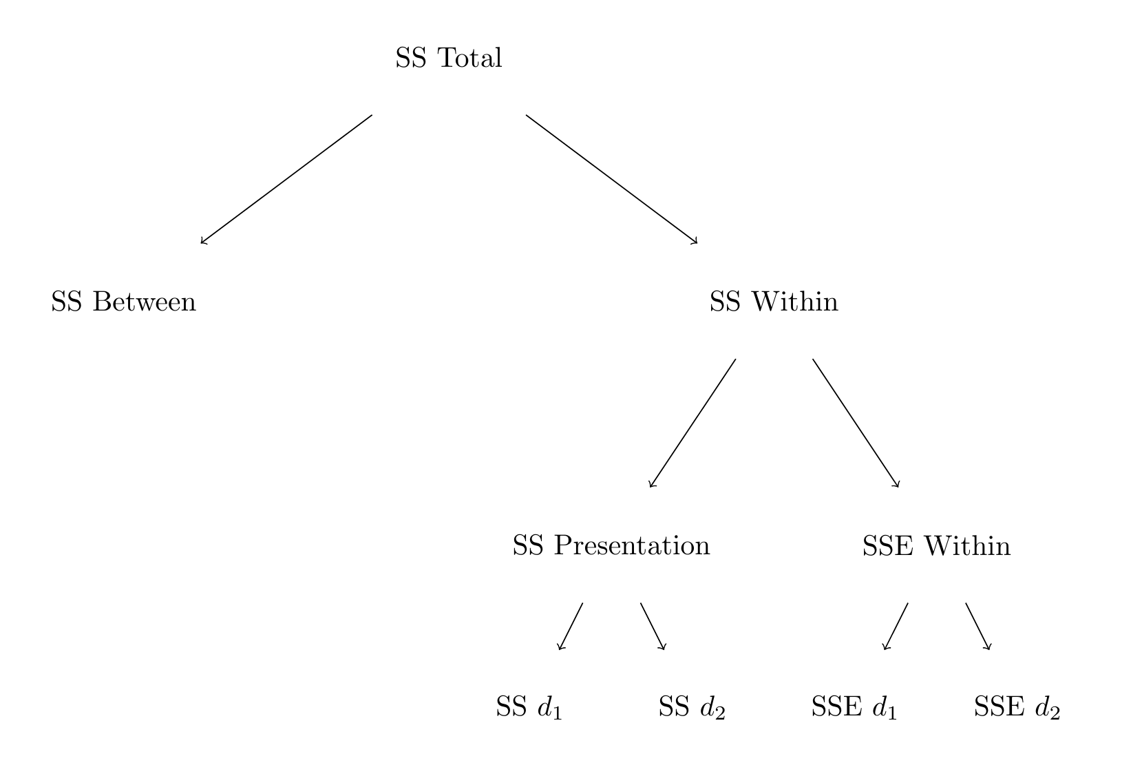
Figure 10.2: Partitioning the total Sum of Squares in a oneway repeated-measures ANOVA.
10.6 A mixed ANOVA with between- and within-subjects effects
Up to now, we just considered the data from the Variant conditions. Having worked out how to perform effective comparisons of the within-subjects conditions, we are now in a position to consider the data from the whole experiment. Whether the other faces in the Similar condition where exact copies of a single photograph, or different photographs of the same person, was a manipulation that varied between participants (i.e., a participant was only assigned to one of these manipulations, not both). The full design of the study is thus a 2 (Version: Identical, Variant) by 3 (Presentation: Alone, Different, Similar) design, where the first factor (Version) varied between, and the last factor (Presentation) varied within participants.
Just like in a “normal” factorial ANOVA, we would like to consider main effects of, and the interaction between, these two experimental manipulations. And just like in a “normal” factorial ANOVA, we will focus on defining contrasts for the main effects, and let the interactions follow from these. We have already defined our \(d_j\) contrasts for the within-subjects effects. There is no need to change these when considering the full experiment, as we still would expect the attractiveness ratings to be different for the Alone conditions compared to the Different and Similar conditions. And while the theory would predict no difference between the Alone condition and the Similar condition when the Version is Identical, we could expect a higher attractiveness rating when the Version is Variant. So, aggregating over the levels of Version, we could still expect a higher attractiveness rating for the Similar conditions. So we just have to define a suitable contrast for the Identical and Variant manipulation. This manipulation only affected the nature of the Similar conditions, and as already indicated, according to the theory, we should expect a higher attractiveness rating when the Version is Variant compared to Identical. So a reasonable contrast code for our single between-subjects manipulation is \(c_1 = (-\tfrac{1}{2},\tfrac{1}{2})\) for the Identical and Variant levels respectively.
Having defined the contrast codes for the main effects, we would normally proceed by defining product-contrasts to reflect the interactions. But in this mixed design, the within-subjects contrasts (\(d\)) are used to transform a set of correlated dependent variables (\(Y\)) in a set of orthogonal dependent variables (\(W\)), whilst the between-subjects contrast (\(c\)) are used to compare different subsets for each of these dependent variables (i.e. because some of the \(W\) values are obtained for the Version: Identical manipulation, and the remainder for the Version: Variant manipulation). Rather than computing product-contrasts, what we will do now is to consider the effect of a contrast-coded predictor \(X_1\) (which takes its values from \(c_1\)) on our three composite variables. As \(W_0\) effectively encodes the marginal mean over all within-subjects conditions, the effect of this contrast-coded predictor on \(W_0\) is equal to a main effect of the between-subjects manipulation. As the within-subjects composite scores encode differences between the within-subjects conditions, an effect of the between-subjects manipulation on such differences is identical to an interaction: The effect of within-subjects manipulations is moderated by the between-subjects manipulation.
To make this less abstract, let’s apply this idea now. Table 10.7 shows the values of the composite variables (computed in the same way as before), as well as the contrast-coded predictor (\(X\)) which codes for Version.
| Participant | Version | Alone | Different | Similar | \(X_1\) | \(W_0\) | \(W_1\) | \(W_2\) |
|---|---|---|---|---|---|---|---|---|
| 1 | Identical | 52.71 | 56.16 | 53.28 | -0.5 | 93.6 | 1.64 | 2.04 |
| 2 | Identical | 52.47 | 55.30 | 55.18 | -0.5 | 94.1 | 2.26 | 0.09 |
| 3 | Identical | 45.89 | 47.91 | 47.74 | -0.5 | 81.7 | 1.58 | 0.12 |
| 4 | Identical | 43.86 | 50.26 | 44.23 | -0.5 | 79.9 | 2.76 | 4.27 |
| 5 | Identical | 37.47 | 34.71 | 37.79 | -0.5 | 63.5 | -1.00 | -2.17 |
| 36 | Variant | 56.32 | 55.92 | 54.30 | 0.5 | 96.2 | -0.99 | 1.15 |
| 37 | Variant | 13.31 | 13.52 | 11.64 | 0.5 | 22.2 | -0.60 | 1.33 |
| 39 | Variant | 49.81 | 49.77 | 51.20 | 0.5 | 87.1 | 0.56 | -1.01 |
| 40 | Variant | 47.10 | 52.48 | 53.19 | 0.5 | 88.2 | 4.68 | -0.50 |
| 41 | Variant | 38.93 | 41.62 | 42.13 | 0.5 | 70.8 | 2.40 | -0.36 |
Let’s start with the tests for \(W_0\), the composite variable for between-subjects effects. We formulate a MODEL G as: \[W_{0,i} = \beta_0 + \beta_1 \times X_{1,i} + \epsilon_{i}\] The main effect of between-subjects contrast \(c_1\) is tested by comparing this model to a MODEL R: \[W_{0,i} = \beta_0 + \epsilon_{i}\] A test of the hypothesis that \(\beta_0 = 0\) is, as usual, obtained by comparing MODEL G to an alternative MODEL R: \[W_{0,i} = \beta_1 \times X_{1,i} + \epsilon_{i}\] The results of these two model comparisons are provided in Table 10.8. We can see that the test of the intercept is significant, tells us that the grand mean of the attractiveness ratings is not likely to equal 0. More interesting is the test of \(X_1\), which compares the marginal means of the attractiveness ratings between the Variant and Identical versions. This test is not significant. Hence, the main effect of Version is not significant: aggregating over the levels of Presentation, there are no differences between the two levels of Version. This is perhaps not overly surprising, as the Version manipulation only concerned the identity of the Similar presentation (whether identical photos or different photos of the same face). The Alone and Different presentations were the same between the Variant and Identical presentation conditions. Therefore, any effect of Version should only affect the attractiveness ratings in the Similar presentation. If the effect on Similar is large enough, this might also show as a difference in the average over Alone, Different, and Similar. But we see here that this is not the case.
| \(\hat{\beta}\) | \(\text{SS}\) | \(\text{df}\) | \(F\) | \(p(\geq F)\) | |
|---|---|---|---|---|---|
| Intercept | 47.675 | 401272 | 1 | 1523.99 | 0.000 |
| \(X_1\) (Variant vs Identical) | -0.499 | 11 | 1 | 0.04 | 0.839 |
| Error | 15008 | 57 |
We now turn to the analysis of the first within-subjects composite variable, \(W_1\). Remember that this variable encodes the first within-subjects contrast \(d_1\), which compares the Different and Similar conditions to the Alone condition. We formulate a MODEL G as: \[W_{1,i} = \beta_0 + \beta_1 \times X_{1,i} + \epsilon_{i}\] As when we conducted a oneway repeated-measures ANOVA, a difference between the Alone vs Different and Similar conditions would show itself through a non-zero intercept. Hence, the main effect of the within-subjects contrast \(d_1\) is tested by comparing this model to a MODEL R where we fix the intercept to 0: \[W_{1,i} = \beta_1 \times X_{1,i} + \epsilon_{i}\] Note that this model allows the value of \(W_1\) to be non-zero through the effect of \(X_1\). Crucially, however, as we are using a sum-to-zero contrast in the construction of \(X_1\) (i.e. the values in \(c_1 = (-\tfrac{1}{2}, \tfrac{1}{2})\) sum to 0), the intercept represents the marginal mean of \(W_1\) over the Identical and Variant versions. In other words, it represents the midpoint of the Identical and Variant versions, or the average effect of the within-subjects contrast \(d_1\) over the levels of the between-subjects factor.
To test whether the effect of \(d_1\) is moderated by \(c_1\), we compare MODEL G to an alternative MODEL R: \[W_{1,i} = \beta_0 + \epsilon_{i}\] If the D + S vs A difference varies over the Identical and Variant groups, then the value of \(W_1\) would be different over these groups. If the D + S vs A difference is not affected by Version, then this last MODEL R would be just as good as MODEL G.
The results of these two model comparisons are provided in Table 10.9. We see a significant and positive intercept. In this model, the intercept is highly relevant, as it reflects a main effect of the \(d_1\) contrast. We thus find evidence that the attractiveness ratings are on average higher in the Different and Similar conditions, compared to the Alone condition. In other words, when presented in the context of a group of faces, a face is rated as more attractive then when presented alone. The test for the slope of \(X_1\), which reflects an interaction between \(d_1\) and \(c_1\), is not significant. Hence, there is no evidence that the D + S vs A contrast is moderated by Version.
| \(\hat{\beta}\) | \(\text{SS}\) | \(\text{df}\) | \(F\) | \(p(\geq F)\) | |
|---|---|---|---|---|---|
| Intercept | 1.29 | 65.8 | 1 | 30.7 | 0.000 |
| \(X_1\) (Variant vs Identical) | 0.01 | 0.0 | 1 | 0.0 | 0.983 |
| Error | 122.2 | 57 |
The procedure for \(W_2\) is the same as for \(W_1\). The results of the two model comparisons are provided in Table 10.10. Here, we see that the intercept is not significant. Hence, there is no evidence of a main effect of \(d_2\), which compares the Different presentation to the Similar presentation. But the slope of \(X_1\), which reflects the \(d_2\) by \(c_1\) interaction, is significant and estimated as negative. There is thus evidence that the difference between the Different and Similar presentation varies over the two versions of the Similar presentation.
| \(\hat{\beta}\) | \(\text{SS}\) | \(\text{df}\) | \(F\) | \(p(\geq F)\) | |
|---|---|---|---|---|---|
| Intercept | 0.396 | 4.62 | 1 | 2.80 | 0.100 |
| \(X_1\) (Variant vs Identical) | -1.173 | 10.12 | 1 | 6.13 | 0.016 |
| Error | 94.05 | 57 |
To interpret the \(d_2\) by \(c_1\) interaction, we can The predicted D - S difference for the Variant condition is: \[\hat{W}_{2,V} = \hat{\beta}_0 + \hat{\beta}_1 \times X_{1,i} = 0.28 + -0.829 \times \tfrac{1}{2} = -0.135\] For the Identical condition, it is \[\hat{W}_{2,I} = 0.28 + -0.829 \times (-\tfrac{1}{2}) = 0.695\] Thus, there appears to be a relatively small difference between presenting a face in the context of a group if different faces, or a group of different images of the same face (Variant version). However, compared to presenting a face within a group of identical photos of the same face (Identical version), a face presented within a group of dissimilar faces is rated as more attractive. This is consistent with the hierarchical encoding hypothesis.
We have considered the effect of Presentation, and the Version by Presentation interaction, through two separate contrasts (\(d_1\) and \(d_2\)). We can also perform omnibus tests of these effects. This is done by summing the relevant SSR, SSE, and df terms. For the main effect of Presentation, we sum the SS terms for the intercept in Table 10.9 and 10.10 to obtain an omnibus SSR for Presentation: \[\text{SSR}(\text{Presentation}) = 65.84 + 4.62 = 70.46\] The error term for this test is computed by summing the SS Error values in these tables: \[\text{SSE}(\text{Presentation}) = 122.25 + 94.05 = 216.3\] The value of \(\text{df}_1\) is the sum of the df terms for the intercept (\(\text{df}_1 = 1 + 1 = 2\)), and the value of \(\text{df}_2\) is the sum of the df terms for the Error (\(\text{df}_2 = 57 + 57 = 114)\). So the resulting \(F\)-statistic is \[F = \frac{70.46/2}{216.3/114} = 18.57\] The exceedence probability of this value in an \(F\)-distribution with \(\text{df}_1 = 2\) and \(\text{df}_2 = 114\) degrees of freedom is \(p(F_{2,114} \geq 18.57) < .001\), and hence this omnibus test is significant.
Similarly, for the Version by Presentation interaction, the omnibus test statistic is computed as \[F = \frac{(0 + 10.12)/2}{(122.25 + 94.05)/114} = 2.67\] The exceedence probability of this value is \(p(F_{2,114} \geq 2.67) = .074\), and hence this omnibus test is not significant. However, we know from our earlier analysis of \(W_2\) that there is evidence for an interaction between \(d_2\) and \(c_1\). Looking at specific contrasts can provide more powerful and interesting tests than an omnibus test whether there is any moderation.
The collated results of all analyses are provided in Table 10.11. This table is separated in a between-subjects part, and a within-subjects part. Relevant omnibus tests and tests for specific contrasts are provided for each. The final row shows the Total Sum of Squares, which is the sum over the between-subjects and within-subjects Sum of Squares. This shows how the Total Sum of Squares is partitioned in the different (between- and within-subjects) effects.
| \(\hat{\beta}\) | \(\text{SS}\) | \(\text{df}\) | \(F\) | \(p(\geq F)\) | |
|---|---|---|---|---|---|
| Between-subjects | 416291.5 | 59 | |||
| Intercept | 47.675 | 401272.2 | 1 | 1523.99 | 0.000 |
| \(c_1\) (Variant vs Identical) | -0.499 | 11.0 | 1 | 0.04 | 0.839 |
| Error between | 15008.3 | 57 | |||
| Within-subjects | 296.9 | 118 | |||
| Presentation | 70.5 | 2 | 18.57 | 0.000 | |
| \(d_1\) (D + S vs A) | 1.295 | 65.8 | 1 | 30.70 | 0.000 |
| Error (\(d_1\)) | 122.2 | 57 | |||
| \(d_2\) (D vs S) | -1.173 | 10.1 | 1 | 6.13 | 0.016 |
| Error (\(d_2\)) | 94.0 | 57 | |||
| Version \(\times\) Presentation | 10.1 | 2 | 2.67 | 0.074 | |
| \(c_1 \times d_1\) | 0.010 | 0.0 | 1 | 0.00 | 0.983 |
| Error (\(c_1 \times d_1\)) | 122.2 | 57 | |||
| \(c_1 \times d_2\) | -1.173 | 10.1 | 1 | 6.13 | 0.016 |
| Error (\(c_1 \times d_2\)) | 94.0 | 57 | |||
| Error within | 216.3 | 114 | |||
| Total | 416588.4 | 177 |
A graphical overview of how the variation in \(Y\) is partitioned in this analysis is provided in Figure 10.3.
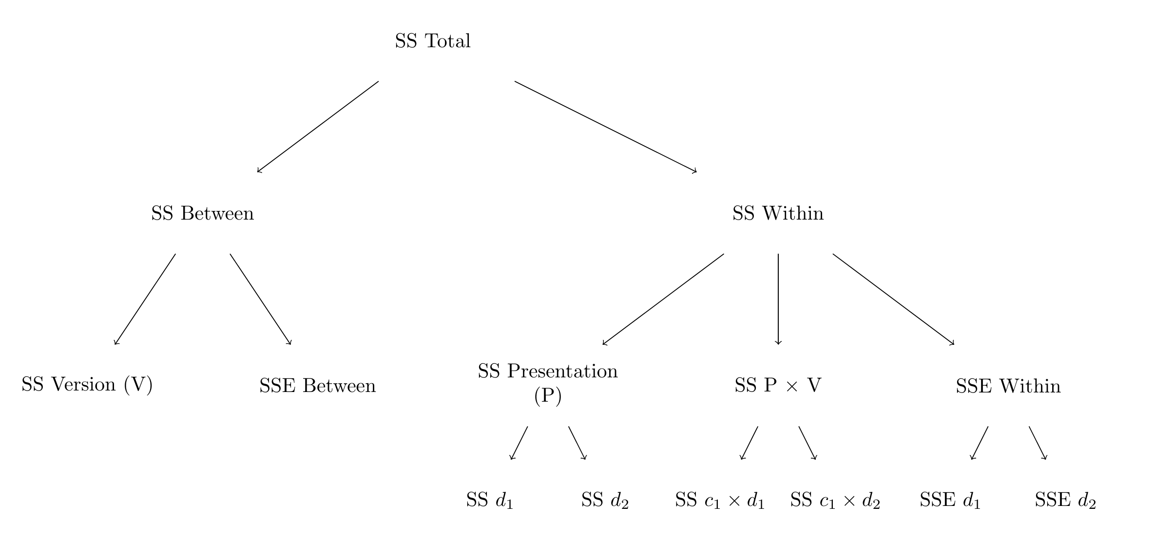
Figure 10.3: Partitioning the total Sum of Squares in a 2 by 3 mixed repeated-measures ANOVA.
10.7 Assumptions
The assumptions for the analyses for each composite variable are the same as for any General Linear Model: the errors are assumed to be independent and Normal-distributed, with a mean of 0 and a constant variance. If the model includes between-subjects groups, then this translates in the assumption that within these groups, each composite score is Normal distributed with the same variance, but a possibly different mean. These assumptions are not guaranteed to hold. However, by focusing on separate analyses of composite scores which, by construction, are orthogonal to each other, there is no immediate reason to suspect a violation of the independence assumption.
When performing omnibus tests of main or interaction effects with a within-subjects component, an additional assumption is required: the assumption of sphericity.
10.7.1 Omnibus tests and sphericity
Omnibus tests involving within-subjects components were performed by aggregating SSR and SSE terms over different models. This is sensible only insofar as the SSE terms are comparable between the models. If the true variances of the errors are substantially different between the models of the within-subjects composite scores, then aggregating them to perform an omnibus test is like treating apples and oranges as the same fruit. As a result, the \(F\)-statistic will not follow the assumed \(F\)-distribution. The omnibus tests are valid when the Data Generating Process is fulfills the requirement of sphericity.
Sphericity means that the variances of all pairwise differences between within-subjects measurements are equal. In our example, there were three within-subjects measurements: the Alone, Different, and Similar attractiveness ratings. As these are ratings by the same person, they are likely to be correlated (the reason for going through the effort in performing a repeated-measures ANOVA). For a more precise definition of sphericity, let’s consider the true variance-covariance matrix of these three measures:
\[\Sigma = \left[ \begin{matrix} \sigma_A^2 & \sigma_{A,D} & \sigma_{A,S} \\ \sigma_{D,A} & \sigma_D^2 & \sigma_{D,S} \\ \sigma_{S,A} & \sigma_{S,D} & \sigma_S^2 \end{matrix} \right]\] Here, \(\sigma^2_A\) represents the true variance of the Alone measurement in the DGP, and \(\sigma_{A,D}\) the true covariance between the Alone and Different measurement. Note that this matrix is symmetric, as the covariance between the Alone and Different measurement is the same as the covariance between the Different and Alone measurement, i.e. \(\sigma_{A,D} = \sigma_{D,A}\). The variance of a pairwise difference between e.g. the Alone and Different measures is \(\sigma_A^2 + \sigma_D^2 - 2 \sigma_{A,D}\), i.e. the sum of the variances of the two variables, minus twice the covariance. Hence, the assumption of sphericity can be stated as: \[\sigma_j^2 + \sigma_k^2 - 2\sigma_{jk} = \sigma_{l}^2 + \sigma_{m}^2 - 2 \sigma_{lm} \quad \quad \text{for all } j,k,l,m\] For example, for our three variables, there are 3 pairwise differences, and hence the assumption is
\[\sigma_A^2 + \sigma_D^2 - 2\sigma_{A,D} = \sigma_{A}^2 + \sigma_{S}^2 - 2 \sigma_{A,S} = \sigma_{D}^2 + \sigma_{S}^2 - 2 \sigma_{D,S}\] If that seems like a complicated and stringent assumption: it is! And it is not that easy to check. Moreover, if there are between-subjects groups, then the variance-covariance matrix should be equal for each of those groups as well. Sphericity holds when a more stringent condition, called compound symmetry holds. Compound symmetry means that all variances are identical to each other (i.e. \(\sigma_A^2 = \sigma_D^2 = \sigma^2_S = \sigma^2\)), and all covariances are identical to each other (i.e. \(\sigma_{A,D} = \sigma_{A,S} = \sigma_{D,S} = \sigma_{\cdot,\cdot}\)). The variance-covariance can then be stated as \[\Sigma = \left[ \begin{matrix} \sigma^2 & \sigma_{\cdot,\cdot} & \sigma_{\cdot,\cdot} \\ \sigma_{\cdot,\cdot} & \sigma^2 & \sigma_{\cdot,\cdot} \\ \sigma_{\cdot,\cdot} & \sigma_{\cdot,\cdot} & \sigma^2 \end{matrix} \right]\]
10.7.2 Correcting for non-sphericity
When the assumption of sphericity does not hold (the assumption is violated) the \(F\)-statistic still (approximately) follows an \(F\) distribution, but with a smaller value for \(\text{df}_1\) and \(\text{df}_2\) than usual. Greenhouse & Geisser (1959) showed that the correct degrees of freedom can be stated as \(\zeta \times \text{df}_1\) and \(\zeta \times \text{df}_2\), where \(0 \geq \zeta \geq 1\) is a correction fraction.26 Whilst the value of \(\zeta\) depends on the true (co)variances underlying the data, it’s value can be estimated. The estimator proposed by Greenhouse & Geisser (1959) is known as the Greenhouse-Geisser estimate, and the corrected degrees of freedom using this estimate as the Greenhouse-Geisser correction. Huynh & Feldt (1976) showed that, if the true value is close to or higher than \(\zeta = 0.75\), the Greenhouse-Geisser correction tends to be too conservative. They suggested a correction which provides an upward-adjusted estimate of \(\zeta\), which will increase the power of the tests. The suggestion is thus to use the Huynh-Feldt correction when the Greenhouse-Geisser estimate of \(\zeta\) is close to or higher than \(\hat{\zeta} = 0.75\).
A statistical test for the assumption of sphericity was developed by Mauchly (1940) and is known as Mauchly’s sphericity test. Whilst routinely provided by statistical software, it is not an ideal test, as it rests strongly on the assumption of normality and it commonly has low power. Rather than only correcting the degrees of freedom after a significant Mauchly test, Howell (2012) suggests to always adjust the degrees of freedom according to the either the Greenhouse-Geisser or Huynh-Feldt correction (whichever is more appropriate given the estimated \(\hat{\zeta}\)). As sphericity is only required for omnibus tests, another consideration is to avoid these omnibus tests, and only focus on tests for individual within-subjects contrasts (Charles M. Judd et al., 2011).
For the present analysis, the Greenhouse-Geisser estimate is \(\hat{\zeta} = 0.982\). This is very close to 1, and hence there is no strong evidence for a violation of sphericity. In this case, that is supported by a non-significant Mauchly test for sphericity, \(W = 0.982\), \(p = .599\). Whilst there is little need to do this in this case, if we were to apply the Greenhouse-Geisser correction for the omnibus test of presentation, we would compare the value of the \(F\)-statistic to an \(F\)-distribution with \(\text{df}_1' = \hat{\zeta} \times \text{df}_1 = 0.982 \times 2 = 1.964\) and \(\text{df}_2' = \hat{\zeta} \times \text{df}_2 = 0.982 \times 114 = 111.971\) degrees of freedom. The exceedence probability is then \(p(F_{1.964,111.971} \geq 18.57) < .001\). The Greenhouse-Geisser corrected test of the Version by Presentation interaction is \(p(F_{1.964,111.971} \geq 2.67) = .075\). As the correction is only minor, neither test result is changed much.
10.8 In practice
Performing a repeated-measures ANOVA is, as you may have noticed, a somewhat laborious affair. It is therefore usually left to statistical software to conduct the various model comparisons. The steps are mostly similar to that of a factorial ANOVA:
Explore the data. For each repeated measure, check the distribution of the scores within each between-subjects condition. Are there outlying or otherwise “strange” observations? If so, you may consider removing these from the dataset. Note that as repeated-measures ANOVA requires complete data for each participant, this implies that you would remove all data from a participant with outlying data.
Define a useful set of contrast codes for the main effects of the within-subjects factors, and any between-subjects factors. Aim for these codes to represent the most important comparisons between the levels of the experimental factors. Then, separately for the within- and between-subjects factors, compute the interaction contrasts as (pairwise, threeway, fourway, …) products of the main-effects contrasts. Compute within-subjects composite scores for all within-subjects effects. Then, for each composite score, estimate a linear model with the relevant contrast-coded predictors for the between-subjects effects. For each of these models, check again for potential issues in the assumptions with e.g. histograms for the residuals and QQ-plots. If there are clear outliers in the data, remove these, and then re-estimate the models.
If you want to compute omnibus tests, check whether the assumption of sphericity is likely to hold. This is best assessed through the Greenhouse-Geisser estimate of the correction factor (which was denoted as \(\hat{\zeta}\) here, but most software will refer to this as \(\hat{\epsilon}\)). If the estimate is far from 1, then the sphericity assumption is likely violated. If the estimate is \(\hat{\zeta} \geq .75\), consider using a Huynh-Feldt correction, rather than Greenhouse-Geisser correction.
If the contrasts do not encode all the comparisons you wish to make, perform follow-up tests with other contrasts. If there are many of these tests, consider correcting for this by using e.g. a Scheffe-adjusted critical value.
Interpret and report the results. When reporting the results, make sure that you include all relevant statistics. For example, one way to write the results of the analysis of Table 10.11, is as follows:
Attractiveness ratings were analysed with a 2 (Version: Identical, Variant) by 3 (Presentation: Alone, Different, Similar) ANOVA, with repeated-measures on the last factor. A Greenhouse-Geisser correction was applied to the degrees of freedom, to correct for any potential problems of non-sphericity. The analysis showed a significant effect of Presentation, \(F(1.96, 111.97) = 18.57\), \(p < .001\), \(\hat{\eta}^2_p = .246\). Contrast analysis showed that attractiveness ratings were higher in the Different and Similar conditions compared to the Alone conditions, \(b = 1.06\), 95% CI \([0.68, 1.44]\), \(t(57) = 5.54\), \(p < .001\). The contrast between the Different and Similar conditions was not significant, \(b = 0.28\), 95% CI \([-0.06, 0.62]\), \(t(57) = 1.67\), \(p = .100\). Whilst the omnibus test for the interaction between Version and Presentation was not significant, \(F(1.96, 111.97) = 2.67\), \(p = .075\), \(\hat{\eta}^2_p = .045\), contrast analysis indicates that the difference between the Different and Similar conditions varied between the two Versions, \(b = -0.83\), 95% CI \([-1.50, -0.16]\), \(t(57) = -2.48\), \(p = .016\). When the Similar condition corresponded to a group of identical photos, the attractiveness ratings were 0.695 points higher in the Different compared to the Similar condition. This difference was only -0.135 when the Similar condition corresponded to a group of different photos of the same individual. The analysis showed no further significant results.
References
Other examples of such clustering in data are when data is collected in group settings, such as students within classrooms, or patients within hospitals. In such situations one could expect again that observations within each cluster (i.e., a specific group, classroom, or hospital) are more similar to each other than observations across clusters.↩︎
Carragher et al. (2019) use different names for the conditions. They call the Different condition the Control condition, the Similar condition the Distractor condition, the Identical condition the Identical-distractors condition, and the Variant condition the Self-distractors condition.↩︎
You might think that it would make sense to use the values \(\left(\tfrac{1}{3}, \tfrac{1}{3}, \tfrac{1}{3}\right)\). Whilst this would give you exactly the same computed values of \(W_{0,i}\), rescaling back to \(Y\) from \(\sqrt{\left(\tfrac{1}{3}\right)^2 + \left(\tfrac{1}{3}\right)^2 + \left(\tfrac{1}{3}\right)^2}\) does not work then. You have to rescale from \(\sqrt{3}\).↩︎
The correction factor is usually denoted by \(\epsilon\), but I’m using \(\zeta\) (“zeta”) as we are already using \(\epsilon\) for the error terms.↩︎