Chapter 11 Structural Equation modelling with lavaan
There are several packages for R which allow you to estimate Structural Equation Models (SEM), including sem (Fox, Nie, and Byrnes 2022), OpenMx (Boker et al. 2023), and lavaan (Rosseel, Jorgensen, and Rockwood 2023). Here, we will focus solely on lavaan.
11.1 Lavaan
The name “lavaan” stands for “latent variable analysis”. It is a package which can estimate a wide-variety of SEM models, including path models without latent variables. It has a convenient and intuitive syntax to define SEM models and it is actively developed. That is why it has perhaps become the go-to R package for SEM analysis. Although the help files in the R package are not overly comprehensive, the lavaan website has a useful tutorial, and I suggest you check this out.
11.1.1 The lavaan model syntax
In lavaan, SEM models can be specified via model formula’s similar to those used in the lm() and glm() functions. However, there are some new operators (relational symbols) used to define (residual) covariances, and latent variables. The table below lists some common expressions in the lavaan syntax.
| Formula | Description |
|---|---|
v =~ y |
latent variable v is defined and measured by y |
v =~ y1 + y2 + y3 |
latent variable v is defined and measured by y1, y2, and y3 |
v =~ 1 + y1 + y2 + y3 |
latent variable v is defined and measured by y1, y2, and y3, with the inclusion of an explicit intercept 1 to model the mean of v |
y ~ x |
y is regressed on x, i.e. a causal relation from x to y |
y ~ b*x |
y is regressed on x, with the slope of x labelled as b |
y ~ x1 + x2 + x3 |
y is regressed on x1, x2 and x3,i.e. causal relations from x1, x2, and x3 to y |
y ~ a*x1 + b*x2 + c*x3 |
regression with labelled slopes |
abc := a*b*c |
define a derived term abc as a function of the model parameters |
y1 ~~ y2 |
(residual) co-variance between y1 and y2 |
y1 ~~ 0*y2 |
fix the (residual) co-variance between y1 and y2 to 0 |
y ~~ y |
(residual) variance for y |
y ~~ 0*y |
fix the (residual) variance for y to 0 |
11.1.2 Model estimation
Under the hood, there is really only a single function used to define and estimate SEM models in the lavaan package, namely the lavaan::lavaan() function. But the lavaan package offers several wrappers around this function to make estimation of common SEM models more convenient. These wrappers set defaults for arguments in the lavaan::lavaan() function that are geared towards particular analyses. Amongst these are the lavaan::sem() function, and the lavaan::cfa() function.
11.1.3 Extracting results
Once a model is estimated, you can use the summary() function on the object returned to get the basic parameter estimates and tests. This function provides the most important results. You can additionally get some of the more widely used fit indices by setting the argument "fit.measures = TRUE". Other functions which can be called on a model fitted by lavaan are:
fitMeasures(): this function returns a long list of model fit measures, only some of which (the more important ones) were discussed in the SDAM bookfitted(): this function returns the model-implied variance-covariance matrix and mean vector.anova(): When provided with a single model, this function returns the results of a likelihood-ratio test of the model against the saturated model. When supplied with multiple models, the function returns likelihood-ratio tests comparing these. This assumes the models are nested!
11.2 Plotting SEM models with the semPlot package
The semPlot package (Epskamp 2022) package provides a convenient way to plot SEM models fitted by lavaan. In principle, all that is needed to plot a lavaan-estimated object mod is a call to semPlot::semPaths(mod). However, the default settings don’t necessarily provide the best looking plots. But the semPlot package is very flexible, and by setting several arguments, it is possible to produce agreeable plots, although it will often require multiple attempts. Important arguments to the semPlot::semPaths() function are
object: for our purposes, this is the object returned bylavaanwhat: this allows you to change the appearance of the arrows based on the parameter estimates. The default ("path") just displays the arrows, but by setting this argument to"est"the linewidth of the arrows reflects the magnitude of the links. For more options, see?semPlot::semPath.whatLabels: This argument sets labels for the arrows. Some of the options are"name"(display the name of the link) and"est"(display the parameter estimates). For more options, see?semPlot::semPath.
11.3 Path models
Path models can be defined and estimated with the lavaan::sem() function. Important arguments for this function are:
model: Astringproviding the model descriptiondata: thedata.framein which all variables in the model description can be foundmeanstructure(passed onto thelavaanfunction): alogicalvalue (TRUEorFALSE) indicating whether the means of the variables should be estimated via intercept termsconditional.x(passed onto thelavaanfunction): alogicalvalue (TRUEorFALSE) indicating whether the model should just consider the conditional distribution of the endogenous variables, conditional upon the exogenous variables.fixed.x(passed onto thelavaanfunction): alogicalvalue (TRUEorFALSE) indicating whether the exogenous variables should be considered as fixed (TRUEby default).estimator(passed onto thelavaanfunction): astringwhich can be"ML"for maximum likelihood,"GLS"for (normal theory) generalized least squares,"WLS"for weighted least squares (sometimes called ADF estimation), or other values. See?lavOptionsfor other possibilities.
Usually, it is fine to stick to the defaults, and just specify the model and data arguments.
11.3.1 Regression models
A simple regression model can be estimated as follows:
# load the data
data("trump2016", package="sdamr")
# exclude the outlying Columbia state
dat <- subset(trump2016,state != "District of Columbia")
# specify the model in lavaan syntax
mod_spec <- 'percent_Trump_votes ~ 1 + hate_groups_per_million'
# estimate the model
library("lavaan")
## This is lavaan 0.6-16
## lavaan is FREE software! Please report any bugs.We can then see the estimates and tests via the summary() function:
## lavaan 0.6.16 ended normally after 1 iteration
##
##   Estimator                                         ML
##   Optimization method                           NLMINB
##   Number of model parameters                         3
##
##   Number of observations                            50
##
## Model Test User Model:
##
##   Test statistic                                 0.000
##   Degrees of freedom                                 0
##
## Parameter Estimates:
##
##   Standard errors                             Standard
##   Information                                 Expected
##   Information saturated (h1) model          Structured
##
## Regressions:
##                         Estimate  Std.Err  z-value  P(>|z|)
##   percent_Trump_votes ~
##     ht_grps_pr_mll         2.300    0.658    3.496    0.000
##
## Intercepts:
##                    Estimate  Std.Err  z-value  P(>|z|)
##    .prcnt_Trmp_vts   42.897    2.361   18.171    0.000
##
## Variances:
##                    Estimate  Std.Err  z-value  P(>|z|)
##    .prcnt_Trmp_vts   80.228   16.046    5.000    0.000
The output of the summary() function first provides information about the way the model was estimated (by maximum likelihood or "ML" by default). Next, under "Model Test User Model" you will find the results of a likelihood-ratio test comparing the model to a saturated model. This test was referred to as the “overall model fit” test in the SDAM book. After this come the parameter estimates, standard errors, and Wald tests. These are displayed in the following order: causal regression effects ("Regressions"), intercepts ("Intercepts"), and (residual) variances (“Variances").
If you want to plot the model, you can use the semPaths() function from the semPlot package:
The default plot is quite basic and does not look so nice. In the following code, I set the arguments layout = tree2 and rotation = 2 to make the plot go from left to right, disable the automatic shortening of variable names by setting nCharNodes = 0, increase the size of the observed (or “manifest”) variables by setting sizeMan=7 and a relatively smaller size for the constant intercepts by setting sizeInt = 4. To display the estimated values as part of the arrows, I also set whatLabels = "est". There are many other tweaks possible, and it pays to play around with the semPaths() function to get the result you want. You should look at the ?semPaths help file to see all the options available. Note that it is useful to rename your variables before calling lavaan::sem() to get better names of the variables in semPlot(), as I will do in the next example.
semPlot::semPaths(fmod, layout="tree2", sizeMan=7, sizeInt = 4, normalize=FALSE,
                  whatLabels="est", width=4, height=1, rotation=2, nCharNodes = 0)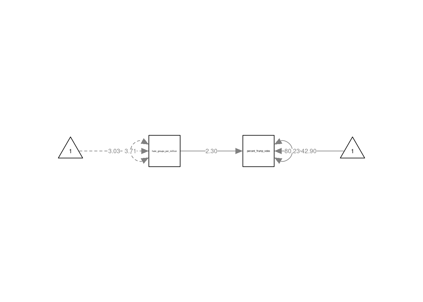
The multiple regression model discussed in the SDAM book is defined in lavaan syntax as
like ~ 1 + attr + sinc + intel + fun + amb
This specifies that like is predicted by (observed) variables attr, sinc, intel, fun, and amb. We also include and intercept via the 1 term in the formula. The model can be specified and estimated as follows:
# load the data
data("speeddate", package="sdamr")
dat <- speeddate
# the following lines are just to get shorter names for the variables
# this is usefull for semPlot. There are better ways to do this though.
dat$like <- dat$other_like
dat$attr <- dat$other_attr
dat$sinc <- dat$other_sinc
dat$intel <- dat$other_intel
dat$fun <- dat$other_fun
dat$amb <- dat$other_amb
# the lavaan model specification
mod_spec <-   'like ~ 1 + attr + sinc + intel + fun + amb'
# estimate the model
fmod <- lavaan::sem(mod_spec, data=dat)
The results can again be obtained with the summary() function. Here we will supply the additional "fit.measures = TRUE" argument to get additional measures of model fit:
## lavaan 0.6.16 ended normally after 1 iteration
##
##   Estimator                                         ML
##   Optimization method                           NLMINB
##   Number of model parameters                         7
##
##                                                   Used       Total
##   Number of observations                          1389        1562
##
## Model Test User Model:
##
##   Test statistic                                 0.000
##   Degrees of freedom                                 0
##
## Model Test Baseline Model:
##
##   Test statistic                              1367.918
##   Degrees of freedom                                 5
##   P-value                                        0.000
##
## User Model versus Baseline Model:
##
##   Comparative Fit Index (CFI)                    1.000
##   Tucker-Lewis Index (TLI)                       1.000
##
## Loglikelihood and Information Criteria:
##
##   Loglikelihood user model (H0)              -2138.891
##   Loglikelihood unrestricted model (H1)      -2138.891
##
##   Akaike (AIC)                                4291.783
##   Bayesian (BIC)                              4328.437
##   Sample-size adjusted Bayesian (SABIC)       4306.201
##
## Root Mean Square Error of Approximation:
##
##   RMSEA                                          0.000
##   90 Percent confidence interval - lower         0.000
##   90 Percent confidence interval - upper         0.000
##   P-value H_0: RMSEA <= 0.050                       NA
##   P-value H_0: RMSEA >= 0.080                       NA
##
## Standardized Root Mean Square Residual:
##
##   SRMR                                           0.000
##
## Parameter Estimates:
##
##   Standard errors                             Standard
##   Information                                 Expected
##   Information saturated (h1) model          Structured
##
## Regressions:
##                    Estimate  Std.Err  z-value  P(>|z|)
##   like ~
##     attr              0.338    0.020   17.007    0.000
##     sinc              0.134    0.028    4.826    0.000
##     intel             0.146    0.032    4.617    0.000
##     fun               0.353    0.023   15.445    0.000
##     amb               0.063    0.024    2.621    0.009
##
## Intercepts:
##                    Estimate  Std.Err  z-value  P(>|z|)
##    .like             -0.753    0.170   -4.428    0.000
##
## Variances:
##                    Estimate  Std.Err  z-value  P(>|z|)
##    .like              1.274    0.048   26.353    0.000
Compared to the usual output, we now also get a likelihood-ratio test against a baseline model ("Model Test Baseline Model"), two fit indices (the CFI and TLI, the latter of which was discussed in the SDAM book), then the AIC and BIC measures, and then two other measures of model fit (the RMSEA and SRMR).
As before, we can get a graphical depiction of the model by using the semPaths() function from the semPlot package. In the code below, I’m additionally setting the argument curvature=3 to make the arrows for the covariances between the exogenous predictors more spread out and easier to see:
semPlot::semPaths(fmod, layout="tree", sizeMan=7, sizeInt = 4, style="ram",
                  residuals=TRUE, rotation=1, intAtSide = FALSE,
                  whatLabels = "est", nCharNodes = 0, curvature=3)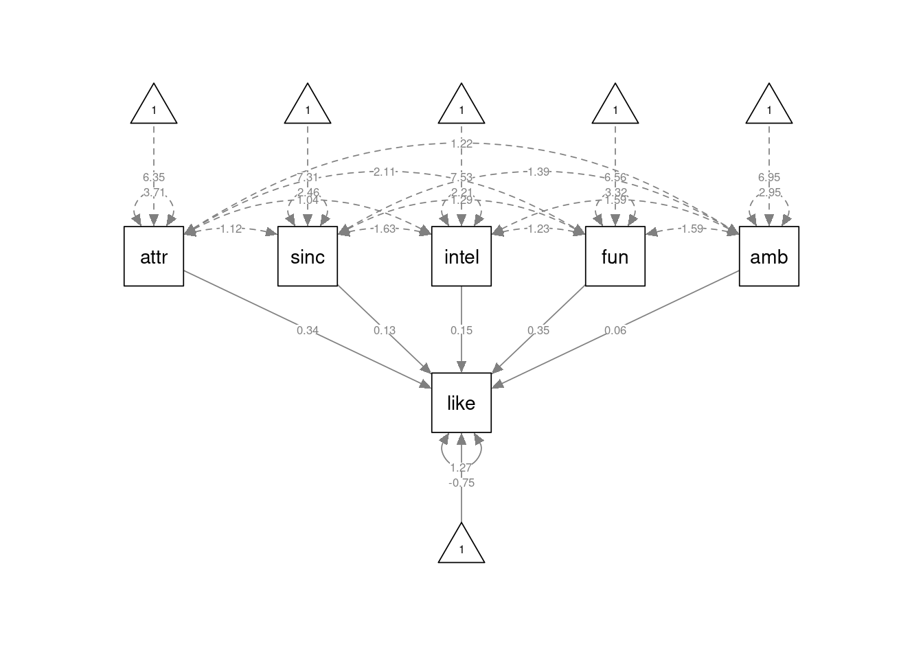
11.3.2 Mediation models
The mediation models concerned the legacy2015 data in the sdamr package, which we should load first:
The Full Mediation model for the relation between legacy motive, intention, and donation, is specified through separate formulas for intention and donation, which are on separate lines of the string that will be supplied to lavaan. We can also explicitly label the regression parameters, which will allow us to compute the indirect effect of legacy on donation
mod1 <-   '
    intention ~ 1 + a*legacy
    donation ~ 1 + b*intention
    ab := a*b # indirect effect of legacy on donation
'
Here, we have specified that intention is caused by legacy, and donation by intention. We have also included an intercept for both endogenous variables. The model can be estimated as usual:
The results are:
## lavaan 0.6.16 ended normally after 1 iteration
##
##   Estimator                                         ML
##   Optimization method                           NLMINB
##   Number of model parameters                         6
##
##   Number of observations                           237
##
## Model Test User Model:
##
##   Test statistic                                 5.989
##   Degrees of freedom                                 1
##   P-value (Chi-square)                           0.014
##
## Model Test Baseline Model:
##
##   Test statistic                                51.556
##   Degrees of freedom                                 3
##   P-value                                        0.000
##
## User Model versus Baseline Model:
##
##   Comparative Fit Index (CFI)                    0.897
##   Tucker-Lewis Index (TLI)                       0.692
##
## Loglikelihood and Information Criteria:
##
##   Loglikelihood user model (H0)               -883.794
##   Loglikelihood unrestricted model (H1)       -880.800
##
##   Akaike (AIC)                                1779.588
##   Bayesian (BIC)                              1800.397
##   Sample-size adjusted Bayesian (SABIC)       1781.379
##
## Root Mean Square Error of Approximation:
##
##   RMSEA                                          0.145
##   90 Percent confidence interval - lower         0.052
##   90 Percent confidence interval - upper         0.266
##   P-value H_0: RMSEA <= 0.050                    0.047
##   P-value H_0: RMSEA >= 0.080                    0.888
##
## Standardized Root Mean Square Residual:
##
##   SRMR                                           0.048
##
## Parameter Estimates:
##
##   Standard errors                             Standard
##   Information                                 Expected
##   Information saturated (h1) model          Structured
##
## Regressions:
##                    Estimate  Std.Err  z-value  P(>|z|)
##   intention ~
##     legacy     (a)    0.267    0.058    4.580    0.000
##   donation ~
##     intention  (b)    1.065    0.205    5.185    0.000
##
## Intercepts:
##                    Estimate  Std.Err  z-value  P(>|z|)
##    .intention         1.785    0.245    7.284    0.000
##    .donation         -0.391    0.619   -0.632    0.528
##
## Variances:
##                    Estimate  Std.Err  z-value  P(>|z|)
##    .intention         0.739    0.068   10.886    0.000
##    .donation          8.047    0.739   10.886    0.000
##
## Defined Parameters:
##                    Estimate  Std.Err  z-value  P(>|z|)
##     ab                0.285    0.083    3.433    0.001
As we have defined a new parameter for the indirect effect of legacy on donation, the results also show the estimate of this new parameter under "Defined Parameters", named ab. We even get a Wald test for the null-hypothesis that the indirect effect is equal to 0 (i.e. no mediation), which is rejected.
A longer list of fit indices can also be obtained via
##                  npar                  fmin                 chisq
##                 6.000                 0.013                 5.989
##                    df                pvalue        baseline.chisq
##                 1.000                 0.014                51.556
##           baseline.df       baseline.pvalue                   cfi
##                 3.000                 0.000                 0.897
##                   tli                  nnfi                   rfi
##                 0.692                 0.692                 0.652
##                   nfi                  pnfi                   ifi
##                 0.884                 0.295                 0.901
##                   rni                  logl     unrestricted.logl
##                 0.897              -883.794              -880.800
##                   aic                   bic                ntotal
##              1779.588              1800.397               237.000
##                  bic2                 rmsea        rmsea.ci.lower
##              1781.379                 0.145                 0.052
##        rmsea.ci.upper        rmsea.ci.level          rmsea.pvalue
##                 0.266                 0.900                 0.047
##        rmsea.close.h0 rmsea.notclose.pvalue     rmsea.notclose.h0
##                 0.050                 0.888                 0.080
##                   rmr            rmr_nomean                  srmr
##                 0.137                 0.168                 0.048
##          srmr_bentler   srmr_bentler_nomean                  crmr
##                 0.048                 0.059                 0.059
##           crmr_nomean            srmr_mplus     srmr_mplus_nomean
##                 0.083                 0.048                 0.059
##                 cn_05                 cn_01                   gfi
##               153.018               263.563                 0.998
##                  agfi                  pgfi                   mfi
##                 0.982                 0.111                 0.990
##                  ecvi
##                 0.076
although this is not as nicely presented as in summary(..., fit.measures=TRUE).
A graphical depiction of the model is obtained as:
semPlot::semPaths(fmod1, layout="tree", sizeMan=7, sizeInt = 4, style="ram",
residuals=TRUE, rotation=2, intAtSide = FALSE,
whatLabels = "est", nCharNodes = 0, normalize = FALSE)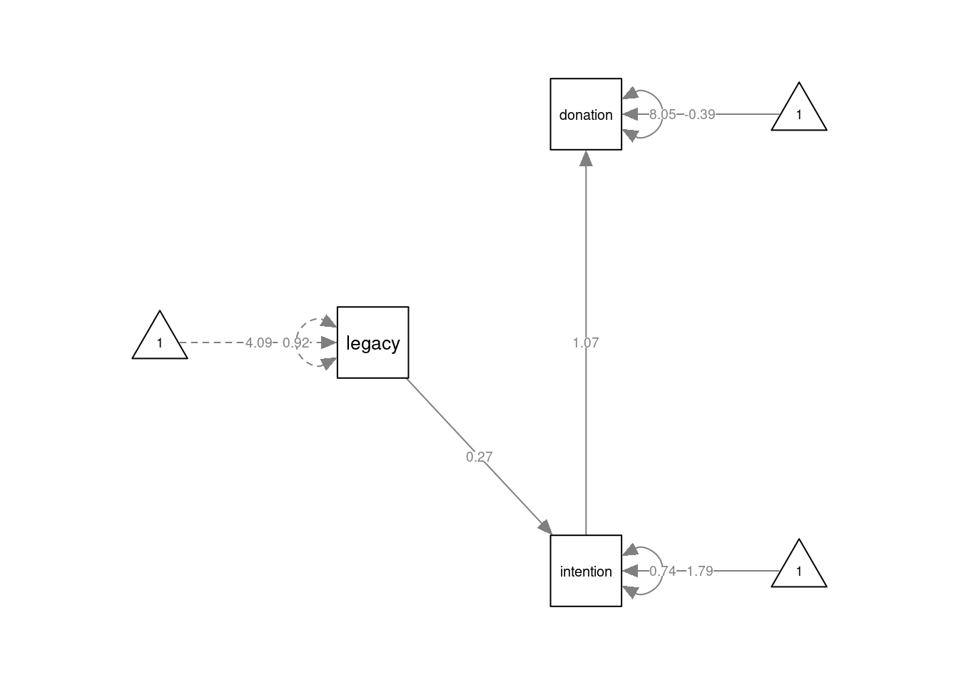 Note I am setting the argument
 "intAtSide = FALSE" to create a better looking plot. You can compare the result with setting "intAtSide = TRUE" to see the effect of this setting.
The Partial Mediation model is specified again by separate formulas for intention and donation, but now we include two predictors for donation:
mod2 <-   '
    intention ~ 1 + a*legacy
    donation ~ 1 + b*intention + c*legacy
    ab := a*b
'
fmod2 <- lavaan::sem(mod2, data=dat)
summary(fmod2, fit.measures=TRUE)
## lavaan 0.6.16 ended normally after 1 iteration
##
## Estimator ML
## Optimization method NLMINB
## Number of model parameters 7
##
## Number of observations 237
##
## Model Test User Model:
##
## Test statistic 0.000
## Degrees of freedom 0
##
## Model Test Baseline Model:
##
## Test statistic 51.556
## Degrees of freedom 3
## P-value 0.000
##
## User Model versus Baseline Model:
##
## Comparative Fit Index (CFI) 1.000
## Tucker-Lewis Index (TLI) 1.000
##
## Loglikelihood and Information Criteria:
##
## Loglikelihood user model (H0) -880.800
## Loglikelihood unrestricted model (H1) -880.800
##
## Akaike (AIC) 1775.599
## Bayesian (BIC) 1799.876
## Sample-size adjusted Bayesian (SABIC) 1777.688
##
## Root Mean Square Error of Approximation:
##
## RMSEA 0.000
## 90 Percent confidence interval - lower 0.000
## 90 Percent confidence interval - upper 0.000
## P-value H_0: RMSEA <= 0.050 NA
## P-value H_0: RMSEA >= 0.080 NA
##
## Standardized Root Mean Square Residual:
##
## SRMR 0.000
##
## Parameter Estimates:
##
## Standard errors Standard
## Information Expected
## Information saturated (h1) model Structured
##
## Regressions:
## Estimate Std.Err z-value P(>|z|)
## intention ~
## legacy (a) 0.267 0.058 4.580 0.000
## donation ~
## intention (b) 0.917 0.212 4.331 0.000
## legacy (c) 0.488 0.198 2.463 0.014
##
## Intercepts:
## Estimate Std.Err z-value P(>|z|)
## .intention 1.785 0.245 7.284 0.000
## .donation -1.961 0.884 -2.220 0.026
##
## Variances:
## Estimate Std.Err z-value P(>|z|)
## .intention 0.739 0.068 10.886 0.000
## .donation 7.846 0.721 10.886 0.000
##
## Defined Parameters:
## Estimate Std.Err z-value P(>|z|)
## ab 0.245 0.078 3.147 0.002semPlot::semPaths(fmod2, layout="tree", sizeMan=7, sizeInt = 5, style="ram",
residuals=TRUE, rotation=2, intAtSide = FALSE, whatLabels = "est",
nCharNodes = 0, normalize=FALSE)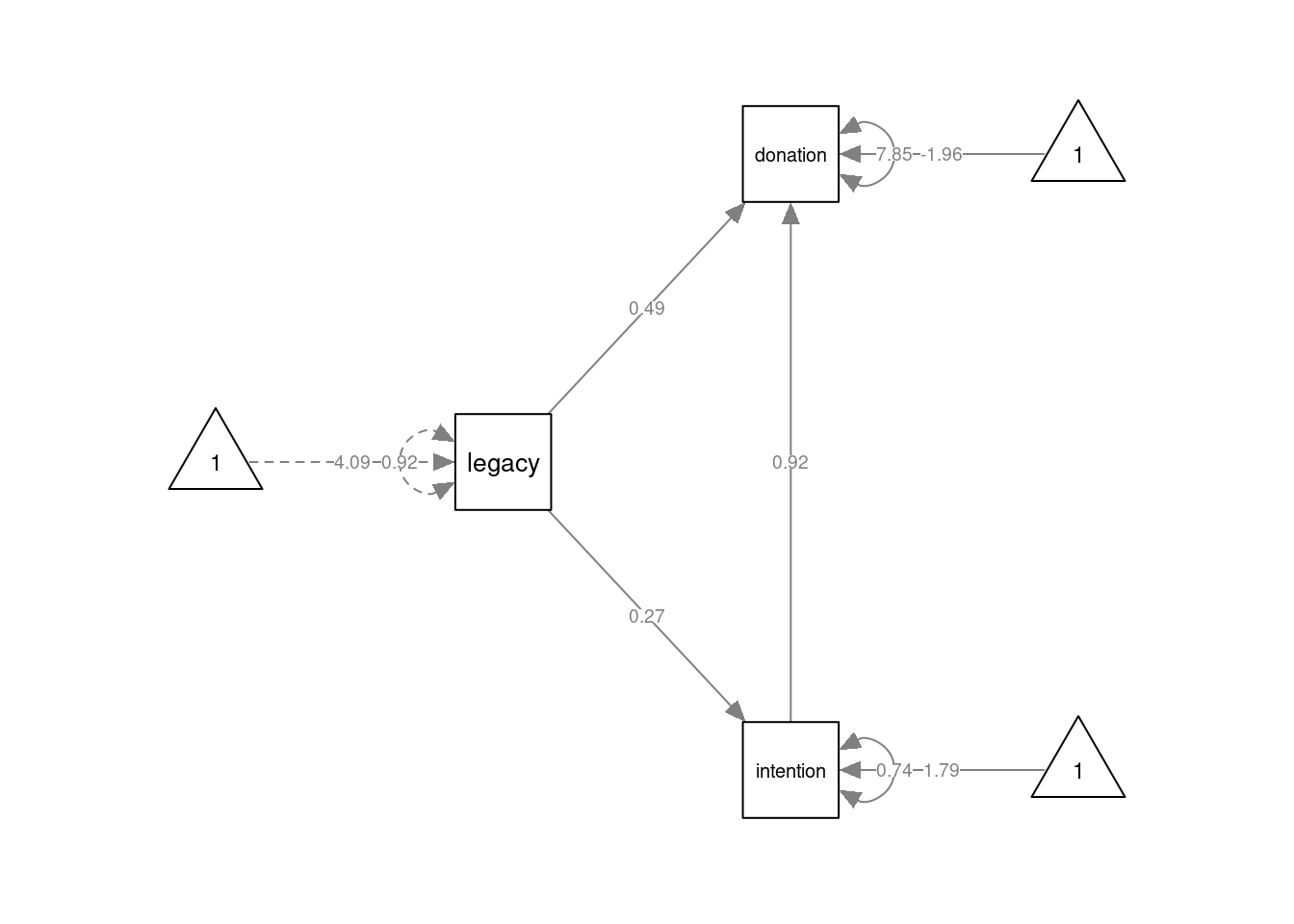 Finally, the Common Cause model can be specified by three formulas. The first two lines concern the regression equations. The third line (
donation ~~ 0*intention) specifies that the (residual) covariance between donation and intention should be fixed to 0.
mod3 <-   '
    intention ~ 1 + legacy
    donation ~ 1 + legacy
    donation ~~ 0*intention
'
fmod3 <- lavaan::sem(mod3, data=dat)
summary(fmod3, fit.measures=TRUE)
## lavaan 0.6.16 ended normally after 1 iteration
##
## Estimator ML
## Optimization method NLMINB
## Number of model parameters 6
##
## Number of observations 237
##
## Model Test User Model:
##
## Test statistic 18.048
## Degrees of freedom 1
## P-value (Chi-square) 0.000
##
## Model Test Baseline Model:
##
## Test statistic 51.556
## Degrees of freedom 3
## P-value 0.000
##
## User Model versus Baseline Model:
##
## Comparative Fit Index (CFI) 0.649
## Tucker-Lewis Index (TLI) -0.053
##
## Loglikelihood and Information Criteria:
##
## Loglikelihood user model (H0) -889.824
## Loglikelihood unrestricted model (H1) -880.800
##
## Akaike (AIC) 1791.648
## Bayesian (BIC) 1812.456
## Sample-size adjusted Bayesian (SABIC) 1793.438
##
## Root Mean Square Error of Approximation:
##
## RMSEA 0.268
## 90 Percent confidence interval - lower 0.169
## 90 Percent confidence interval - upper 0.383
## P-value H_0: RMSEA <= 0.050 0.000
## P-value H_0: RMSEA >= 0.080 0.999
##
## Standardized Root Mean Square Residual:
##
## SRMR 0.084
##
## Parameter Estimates:
##
## Standard errors Standard
## Information Expected
## Information saturated (h1) model Structured
##
## Regressions:
## Estimate Std.Err z-value P(>|z|)
## intention ~
## legacy 0.267 0.058 4.580 0.000
## donation ~
## legacy 0.733 0.197 3.714 0.000
##
## Covariances:
## Estimate Std.Err z-value P(>|z|)
## .intention ~~
## .donation 0.000
##
## Intercepts:
## Estimate Std.Err z-value P(>|z|)
## .intention 1.785 0.245 7.284 0.000
## .donation -0.325 0.830 -0.392 0.695
##
## Variances:
## Estimate Std.Err z-value P(>|z|)
## .intention 0.739 0.068 10.886 0.000
## .donation 8.467 0.778 10.886 0.000semPlot::semPaths(fmod3, layout="tree", sizeMan=7, sizeInt = 5, style="ram",
residuals=TRUE, rotation=2, intAtSide = FALSE,
whatLabels = "est", nCharNodes = 0, normalize=FALSE)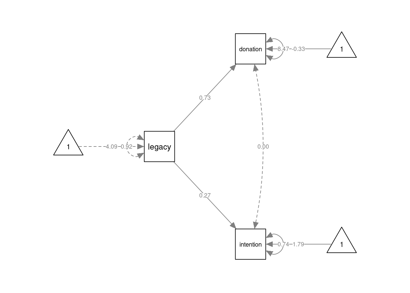 We can obtain likelihood-ratio tests for nested models with the
 anova() function. For sample, we can compare the Full Mediation model to the Partial Mediation model with:
##
## Chi-Squared Difference Test
##
##       Df    AIC    BIC  Chisq Chisq diff   RMSEA Df diff Pr(>Chisq)
## fmod2  0 1775.6 1799.9 0.0000
## fmod1  1 1779.6 1800.4 5.9889     5.9889 0.14509       1     0.0144 *
## ---
## Signif. codes:  0 '***' 0.001 '**' 0.01 '*' 0.05 '.' 0.1 ' ' 1
And we can compare the Common Cause model to the Partial Mediation model with:
##
## Chi-Squared Difference Test
##
##       Df    AIC    BIC  Chisq Chisq diff   RMSEA Df diff Pr(>Chisq)
## fmod2  0 1775.6 1799.9  0.000
## fmod3  1 1791.7 1812.5 18.048     18.048 0.26821       1  2.154e-05 ***
## ---
## Signif. codes:  0 '***' 0.001 '**' 0.01 '*' 0.05 '.' 0.1 ' ' 1
As the Partial Mediation model is saturated, these tests are equivalent to the model fit tests reported by the summary() function for fmod1 and fmod3.
11.3.3 A more complex path model
More complex path models can be estimated by including more formula’s in the model specification. For example:
mod_complex <-   '
    belief ~ 1 + education
    legacy ~ 1 + age
    income ~ 1 + age + education
    intention ~ 1 + belief + legacy + income
    donation ~ 1 + intention + income
'
fmod_complex <- lavaan::sem(mod_complex, data=legacy2015)
summary(fmod_complex)
## lavaan 0.6.16 ended normally after 1 iteration
##
## Estimator ML
## Optimization method NLMINB
## Number of model parameters 19
##
## Used Total
## Number of observations 224 237
##
## Model Test User Model:
##
## Test statistic 41.291
## Degrees of freedom 11
## P-value (Chi-square) 0.000
##
## Parameter Estimates:
##
## Standard errors Standard
## Information Expected
## Information saturated (h1) model Structured
##
## Regressions:
## Estimate Std.Err z-value P(>|z|)
## belief ~
## education 0.132 0.048 2.723 0.006
## legacy ~
## age -0.006 0.005 -1.120 0.263
## income ~
## age 0.002 0.009 0.254 0.800
## education 0.384 0.102 3.757 0.000
## intention ~
## belief 0.738 0.064 11.615 0.000
## legacy 0.123 0.049 2.522 0.012
## income -0.080 0.030 -2.710 0.007
## donation ~
## intention 1.098 0.213 5.152 0.000
## income 0.257 0.121 2.113 0.035
##
## Intercepts:
## Estimate Std.Err z-value P(>|z|)
## .belief 4.416 0.222 19.912 0.000
## .legacy 4.322 0.208 20.773 0.000
## .income 1.220 0.569 2.143 0.032
## .intention -1.077 0.386 -2.790 0.005
## .donation -1.232 0.774 -1.592 0.111
##
## Variances:
## Estimate Std.Err z-value P(>|z|)
## .belief 0.520 0.049 10.583 0.000
## .legacy 0.906 0.086 10.583 0.000
## .income 2.318 0.219 10.583 0.000
## .intention 0.485 0.046 10.583 0.000
## .donation 8.039 0.760 10.583 0.000To plot complex models like this, it may be useful to hide the constant (intercept) terms, which is achieved by setting "intercepts" = FALSE in the call to semPlot::semPaths():
semPlot::semPaths(fmod_complex, layout="tree2", sizeMan=7, sizeInt = 5,
                  style="ram", intercepts=FALSE, residuals=TRUE, rotation=2,
                  intAtSide = FALSE, whatLabels = "est", nCharNodes = 0,
                  normalize=FALSE)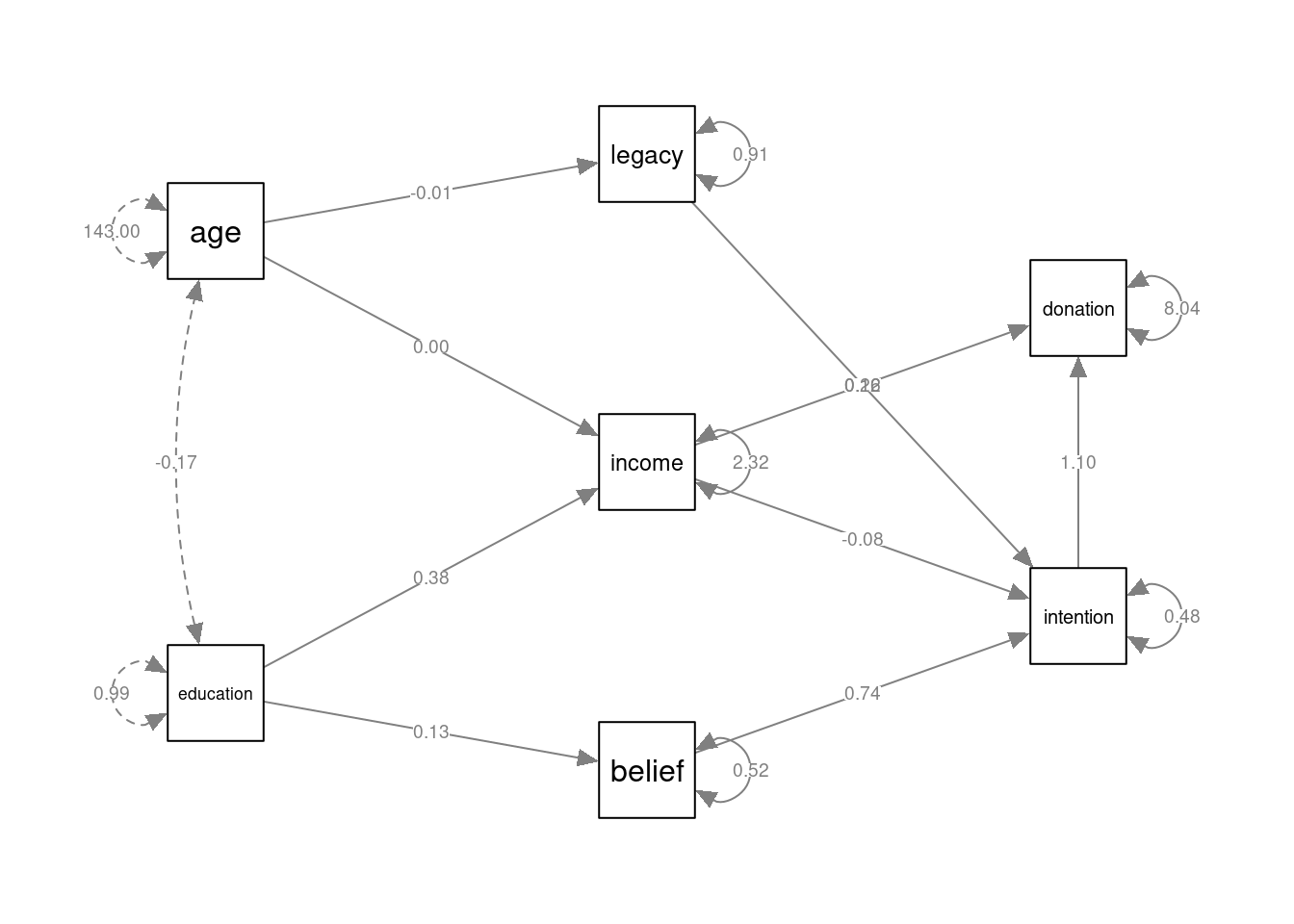
11.4 Modification indices
Modification indices can be obtained with the modificationIndices() from the lavaan package. Modification indices estimated the (positive) change in overall model fit when estimating, rather than fixing a parameter to a specific value. This change is provided in terms of the Chi-squared statistic (\(X^2\)), which under the null-hypothesis is distributed with \(\text{df}=1\).
For a given model, there are generally a lot of these indices, as many parameters might be fixed. By default, the lavaan::modificationIndices() functions also displays the expected change in the parameter value, including various standardized measures of such change. By setting the argument standardized = FALSE, these values are excluded, providing slightly more succinct output. An example providing all modification indices for the last path model above is given in the code below. Be ready for lots of output!
##          lhs op       rhs     mi    epc
## 20 education ~~ education  0.000  0.000
## 21 education ~~       age  0.000  0.000
## 25    belief ~~    legacy 13.545  0.169
## 26    belief ~~    income  1.670  0.095
## 27    belief ~~ intention  0.006 -0.015
## 28    belief ~~  donation  3.559  0.322
## 29    legacy ~~    income  1.952  0.135
## 30    legacy ~~ intention  7.674  1.644
## 31    legacy ~~  donation  5.218  0.415
## 32    income ~~ intention  0.074 -0.081
## 33    income ~~  donation  1.673 -1.539
## 34 intention ~~  donation  7.590 -0.584
## 35    belief  ~    legacy 13.986  0.189
## 36    belief  ~    income  1.629  0.040
## 37    belief  ~ intention  1.719  0.303
## 38    belief  ~  donation  4.915  0.047
## 39    belief  ~       age  0.872 -0.004
## 40    legacy  ~    belief 15.995  0.347
## 41    legacy  ~    income  3.496  0.076
## 42    legacy  ~ intention 14.055  0.431
## 43    legacy  ~  donation 10.703  0.072
## 44    legacy  ~ education  4.470  0.135
## 45    income  ~    belief  1.670  0.182
## 46    income  ~    legacy  1.952  0.149
## 47    income  ~ intention  1.998  0.252
## 48    income  ~  donation  0.000 -0.001
## 49 intention  ~  donation  7.590 -0.073
## 50 intention  ~ education  0.006  0.004
## 51 intention  ~       age  7.674  0.011
## 52  donation  ~    belief  4.661  0.704
## 53  donation  ~    legacy  5.253  0.459
## 54  donation  ~ education  1.711  0.258
## 55  donation  ~       age  0.034 -0.003
## 56 education  ~    belief  0.349 -2.482
## 57 education  ~    legacy  4.420  0.146
## 58 education  ~    income  0.000  0.000
## 59 education  ~ intention  0.223  0.046
## 60 education  ~  donation  1.914  0.032
## 61 education  ~       age  0.000  0.000
## 62       age  ~    belief  0.817 -0.969
## 64       age  ~    income  0.000  0.000
## 65       age  ~ intention  2.631  1.469
## 66       age  ~  donation  0.134  0.097
## 67       age  ~ education  0.000  0.000
In the resulting table, the column lhs stands for the “dependent variable” in a relation, and rhs for the “independent variable”, whilst the op stands for the type of relation. The column mi reports the expected chi-square change from estimating the parameter corresponding to the relation between rhs and lhs, whilst epc stands for the expected parameter change (i.e. the change from a fixed-to-zero value 0 to the estimated value).
The argument minimum.value can be used to exclude modification indices below a certain value. For example, we might only be interested in modification indices above 5. In addition, it can be useful to order the output by the magnitude of the modification index, showing the most promising parameters first, This can be obtained by setting the argument sort. to TRUE. Below, we do both to get some idea of possible parameters which might be useful to allow to be estimated. This still provides many modification indices, but at least a few less.
##          lhs op       rhs     mi    epc
## 40    legacy  ~    belief 15.995  0.347
## 42    legacy  ~ intention 14.055  0.431
## 35    belief  ~    legacy 13.986  0.189
## 25    belief ~~    legacy 13.545  0.169
## 43    legacy  ~  donation 10.703  0.072
## 30    legacy ~~ intention  7.674  1.644
## 51 intention  ~       age  7.674  0.011
## 49 intention  ~  donation  7.590 -0.073
## 34 intention ~~  donation  7.590 -0.584
## 53  donation  ~    legacy  5.253  0.459
## 31    legacy ~~  donation  5.218  0.415
An important thing to remember when inspecting these modification indices is that each indicates what would happen to the model if a single parameter is estimated rather than fixed. If you would include e.g. a direct path from belief to legacy , as suggested by the highest modification index, then the model would change and therefore the resulting modification indices of that modified model would be different from those of the current model. Hence, it does not necessarily make sense to change all fixed variables according to the modification indices. If you are willing to change a model in an exploratory way, this should be a sequential procedure, adding one estimated parameter and then inspecting the modification indices again. It is also important to keep in mind that such sequential procedures don’t necessarily lead to the best possible model. Theoretical concerns should outweigh modification indices.
11.5 Confirmatory factor analysis
In the following, we will use the bfi data included in the psychTools package as an example.
##       A1 A2 A3 A4 A5 C1 C2 C3 C4 C5 E1 E2 E3 E4 E5 N1 N2 N3 N4 N5 O1 O2 O3 O4
## 61617  2  4  3  4  4  2  3  3  4  4  3  3  3  4  4  3  4  2  2  3  3  6  3  4
## 61618  2  4  5  2  5  5  4  4  3  4  1  1  6  4  3  3  3  3  5  5  4  2  4  3
## 61620  5  4  5  4  4  4  5  4  2  5  2  4  4  4  5  4  5  4  2  3  4  2  5  5
## 61621  4  4  6  5  5  4  4  3  5  5  5  3  4  4  4  2  5  2  4  1  3  3  4  3
## 61622  2  3  3  4  5  4  4  5  3  2  2  2  5  4  5  2  3  4  4  3  3  3  4  3
## 61623  6  6  5  6  5  6  6  6  1  3  2  1  6  5  6  3  5  2  2  3  4  3  5  6
##       O5 gender education age
## 61617  3      1        NA  16
## 61618  3      2        NA  18
## 61620  2      2        NA  17
## 61621  5      2        NA  17
## 61622  3      1        NA  17
## 61623  1      2         3  21
Confirmatory Factor Analysis (CFA) can be performed via the cfa() function in the lavaan package. This function is very much like the sem() function, but uses different defaults. A main thing to supply is a specification of the model in the lavaan syntax.
Latent variables (the factors) can be specified with the =~ operator. On the right-hand side of this operator, you can specify a name for the factor, and on the left hand side you can specify which observed variables load onto the factor (i.e. which observed variables are partially caused by the factor), separated by a “+” sign. For instance, the line
agreeableness =~ A1 + A2 + A3 + A4 + A5specifies that a latent factor called “agreeableness” accounts for shared variation in observed variables A1, A2, A3, A4, and A5.
The following code specifies a CFA with a simple structure, in the sense that each observed variable only loads onto one factor:
bfi_cfa_spec <- '
  # factor specification
    agreeableness =~ A1 + A2 + A3 + A4 + A5
    conscientiousness =~  C1 + C2 + C3 + C4 + C5
    extraversion =~  E1 + E2 + E3 + E4 + E5
    neuroticism =~ N1 + N2 + N3 + N4 + N5
    openness =~ O1 + O2 + O3 + O4 + O5
'
Using this lavaan model specification, the model can be estimated with the lavaan::cfa() function:
Having estimated the model, we can obtain parameter estimates and tests via the summary function:
## lavaan 0.6.16 ended normally after 55 iterations
##
##   Estimator                                         ML
##   Optimization method                           NLMINB
##   Number of model parameters                        60
##
##                                                   Used       Total
##   Number of observations                          2436        2800
##
## Model Test User Model:
##
##   Test statistic                              4165.467
##   Degrees of freedom                               265
##   P-value (Chi-square)                           0.000
##
## Model Test Baseline Model:
##
##   Test statistic                             18222.116
##   Degrees of freedom                               300
##   P-value                                        0.000
##
## User Model versus Baseline Model:
##
##   Comparative Fit Index (CFI)                    0.782
##   Tucker-Lewis Index (TLI)                       0.754
##
## Loglikelihood and Information Criteria:
##
##   Loglikelihood user model (H0)             -99840.238
##   Loglikelihood unrestricted model (H1)     -97757.504
##
##   Akaike (AIC)                              199800.476
##   Bayesian (BIC)                            200148.363
##   Sample-size adjusted Bayesian (SABIC)     199957.729
##
## Root Mean Square Error of Approximation:
##
##   RMSEA                                          0.078
##   90 Percent confidence interval - lower         0.076
##   90 Percent confidence interval - upper         0.080
##   P-value H_0: RMSEA <= 0.050                    0.000
##   P-value H_0: RMSEA >= 0.080                    0.037
##
## Standardized Root Mean Square Residual:
##
##   SRMR                                           0.075
##
## Parameter Estimates:
##
##   Standard errors                             Standard
##   Information                                 Expected
##   Information saturated (h1) model          Structured
##
## Latent Variables:
##                        Estimate  Std.Err  z-value  P(>|z|)
##   agreeableness =~
##     A1                    1.000
##     A2                   -1.579    0.108  -14.650    0.000
##     A3                   -2.030    0.134  -15.093    0.000
##     A4                   -1.564    0.115  -13.616    0.000
##     A5                   -1.804    0.121  -14.852    0.000
##   conscientiousness =~
##     C1                    1.000
##     C2                    1.148    0.057   20.152    0.000
##     C3                    1.036    0.054   19.172    0.000
##     C4                   -1.421    0.065  -21.924    0.000
##     C5                   -1.489    0.072  -20.694    0.000
##   extraversion =~
##     E1                    1.000
##     E2                    1.226    0.051   23.899    0.000
##     E3                   -0.921    0.041  -22.431    0.000
##     E4                   -1.121    0.047  -23.977    0.000
##     E5                   -0.808    0.039  -20.648    0.000
##   neuroticism =~
##     N1                    1.000
##     N2                    0.947    0.024   39.899    0.000
##     N3                    0.884    0.025   35.919    0.000
##     N4                    0.692    0.025   27.753    0.000
##     N5                    0.628    0.026   24.027    0.000
##   openness =~
##     O1                    1.000
##     O2                   -1.020    0.068  -14.962    0.000
##     O3                    1.373    0.072   18.942    0.000
##     O4                    0.437    0.048    9.160    0.000
##     O5                   -0.960    0.060  -16.056    0.000
##
## Covariances:
##                        Estimate  Std.Err  z-value  P(>|z|)
##   agreeableness ~~
##     conscientisnss       -0.110    0.012   -9.254    0.000
##     extraversion          0.304    0.025   12.293    0.000
##     neuroticism           0.141    0.018    7.712    0.000
##     openness             -0.093    0.011   -8.446    0.000
##   conscientiousness ~~
##     extraversion         -0.224    0.020  -11.121    0.000
##     neuroticism          -0.250    0.025  -10.117    0.000
##     openness              0.130    0.014    9.190    0.000
##   extraversion ~~
##     neuroticism           0.292    0.032    9.131    0.000
##     openness             -0.265    0.021  -12.347    0.000
##   neuroticism ~~
##     openness             -0.093    0.022   -4.138    0.000
##
## Variances:
##                    Estimate  Std.Err  z-value  P(>|z|)
##    .A1                1.745    0.052   33.725    0.000
##    .A2                0.807    0.028   28.396    0.000
##    .A3                0.754    0.032   23.339    0.000
##    .A4                1.632    0.051   31.796    0.000
##    .A5                0.852    0.032   26.800    0.000
##    .C1                1.063    0.035   30.073    0.000
##    .C2                1.130    0.039   28.890    0.000
##    .C3                1.170    0.039   30.194    0.000
##    .C4                0.960    0.040   24.016    0.000
##    .C5                1.640    0.059   27.907    0.000
##    .E1                1.814    0.058   31.047    0.000
##    .E2                1.332    0.049   26.928    0.000
##    .E3                1.108    0.038   29.522    0.000
##    .E4                1.088    0.041   26.732    0.000
##    .E5                1.251    0.040   31.258    0.000
##    .N1                0.793    0.037   21.575    0.000
##    .N2                0.836    0.036   23.458    0.000
##    .N3                1.222    0.043   28.271    0.000
##    .N4                1.654    0.052   31.977    0.000
##    .N5                1.969    0.060   32.889    0.000
##    .O1                0.865    0.032   27.216    0.000
##    .O2                1.990    0.063   31.618    0.000
##    .O3                0.691    0.039   17.717    0.000
##    .O4                1.346    0.040   34.036    0.000
##    .O5                1.380    0.045   30.662    0.000
##     agreeableness     0.234    0.030    7.839    0.000
##     conscientisnss    0.463    0.036   12.810    0.000
##     extraversion      0.846    0.062   13.693    0.000
##     neuroticism       1.689    0.073   23.034    0.000
##     openness          0.404    0.033   12.156    0.000
Note that for the summary() function to work, you need to have loaded the lavaan package with library(lavaan).
A plot can again be obtained with the semPlot::semPaths() function
semPlot::semPaths(bfi_cfa, layout="tree", sizeMan=3, residuals=TRUE, rotation=1, whatLabels = "est", nCharNodes = 5, normalize=TRUE, width=12, height=6)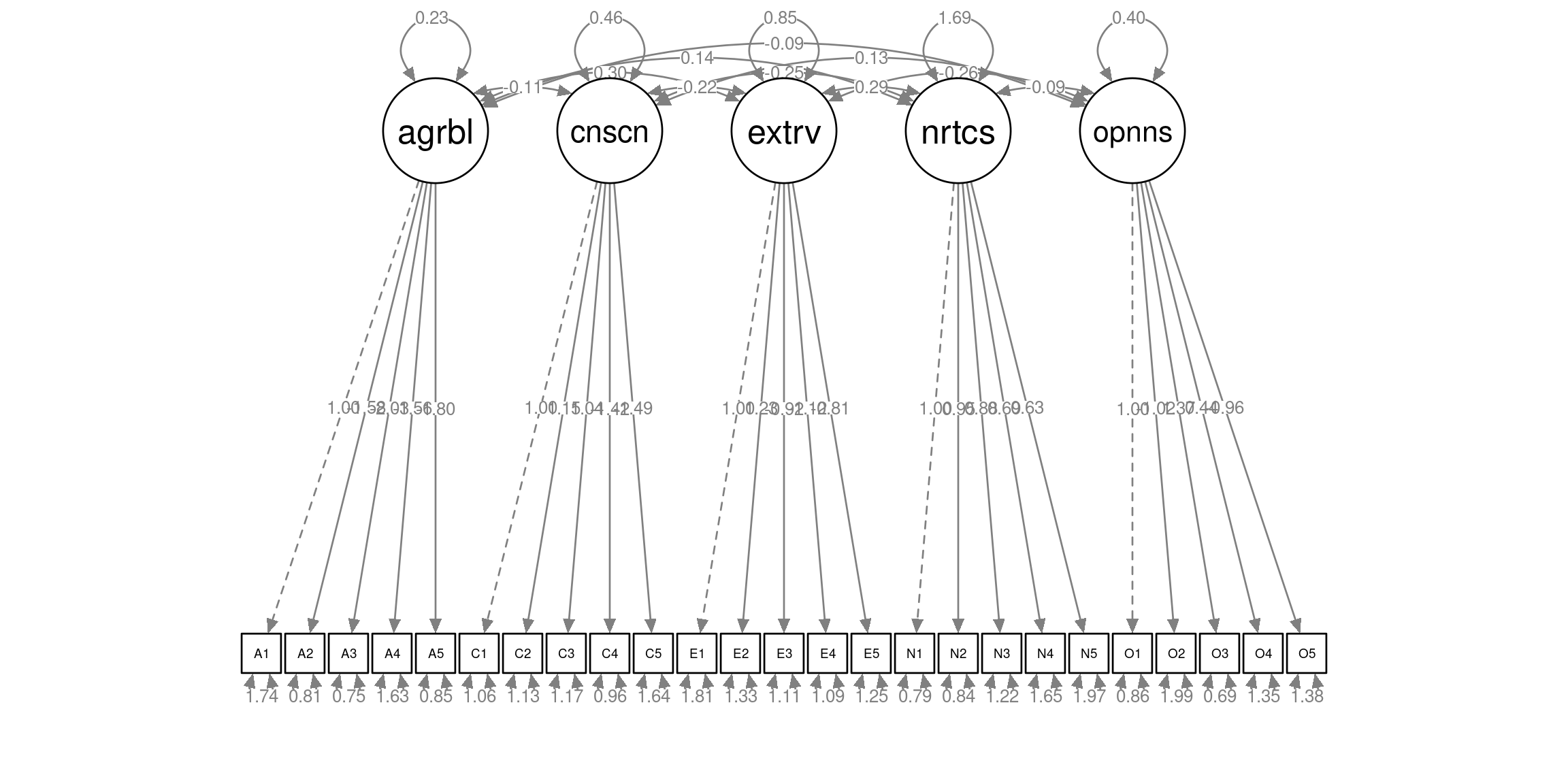
Note that by default, factors are allowed to correlate. If you want to obtain a solution for uncorrelated factors, you need to explicitly fix the covariances between the factors to 0. This can be done via the ~~ operator, and multiplying the factors on the right-hand side of this operator to 0. For example, the line
agreeableness ~~ 0*conscientiousness + 0*extraversion + 0*neuroticism + 0*opennessspecifies that the covariance between factor agreeableness and conscientiousness is 0 (agreeableness ~~ 0*conscientiousness), as well as the covariance between factor agreeableness and extraversion, neuroticism, and openness. You should only fix a covariance once, so you should not also have a line which states e.g.
conscientiousness ~~ 0*agreeablenessas this would lead to an error. The model specification below fixes the covariance for all pairs of factors to 0:
bfi_cfa2_spec <-   '
  # factor specification
    agreeableness =~ A1 + A2 + A3 + A4 + A5
    conscientiousness =~  C1 + C2 + C3 + C4 + C5
    extraversion =~  E1 + E2 + E3 + E4 + E5
    neuroticism =~ N1 + N2 + N3 + N4 + N5
    openness =~ O1 + O2 + O3 + O4 + O5
  # fix factor covariances to 0
    agreeableness ~~ 0*conscientiousness + 0*extraversion + 0*neuroticism + 0*openness
    conscientiousness ~~ 0*extraversion + 0*neuroticism + 0*openness
    extraversion ~~ 0*neuroticism + 0*openness
    neuroticism ~~ 0*openness
'
Using this specification, the results are:
## lavaan 0.6.16 ended normally after 53 iterations
##
##   Estimator                                         ML
##   Optimization method                           NLMINB
##   Number of model parameters                        50
##
##                                                   Used       Total
##   Number of observations                          2436        2800
##
## Model Test User Model:
##
##   Test statistic                              5639.709
##   Degrees of freedom                               275
##   P-value (Chi-square)                           0.000
##
## Model Test Baseline Model:
##
##   Test statistic                             18222.116
##   Degrees of freedom                               300
##   P-value                                        0.000
##
## User Model versus Baseline Model:
##
##   Comparative Fit Index (CFI)                    0.701
##   Tucker-Lewis Index (TLI)                       0.673
##
## Loglikelihood and Information Criteria:
##
##   Loglikelihood user model (H0)            -100577.359
##   Loglikelihood unrestricted model (H1)     -97757.504
##
##   Akaike (AIC)                              201254.718
##   Bayesian (BIC)                            201544.623
##   Sample-size adjusted Bayesian (SABIC)     201385.762
##
## Root Mean Square Error of Approximation:
##
##   RMSEA                                          0.089
##   90 Percent confidence interval - lower         0.087
##   90 Percent confidence interval - upper         0.092
##   P-value H_0: RMSEA <= 0.050                    0.000
##   P-value H_0: RMSEA >= 0.080                    1.000
##
## Standardized Root Mean Square Residual:
##
##   SRMR                                           0.138
##
## Parameter Estimates:
##
##   Standard errors                             Standard
##   Information                                 Expected
##   Information saturated (h1) model          Structured
##
## Latent Variables:
##                        Estimate  Std.Err  z-value  P(>|z|)
##   agreeableness =~
##     A1                    1.000
##     A2                   -1.468    0.092  -15.885    0.000
##     A3                   -1.887    0.116  -16.273    0.000
##     A4                   -1.394    0.097  -14.400    0.000
##     A5                   -1.502    0.096  -15.658    0.000
##   conscientiousness =~
##     C1                    1.000
##     C2                    1.172    0.057   20.409    0.000
##     C3                    1.047    0.054   19.347    0.000
##     C4                   -1.377    0.064  -21.526    0.000
##     C5                   -1.403    0.070  -20.029    0.000
##   extraversion =~
##     E1                    1.000
##     E2                    1.205    0.048   25.012    0.000
##     E3                   -0.785    0.036  -21.573    0.000
##     E4                   -1.034    0.042  -24.402    0.000
##     E5                   -0.713    0.035  -20.195    0.000
##   neuroticism =~
##     N1                    1.000
##     N2                    0.947    0.024   40.245    0.000
##     N3                    0.873    0.024   35.898    0.000
##     N4                    0.665    0.025   26.891    0.000
##     N5                    0.616    0.026   23.814    0.000
##   openness =~
##     O1                    1.000
##     O2                   -1.165    0.077  -15.042    0.000
##     O3                    1.248    0.074   16.878    0.000
##     O4                    0.551    0.052   10.515    0.000
##     O5                   -1.106    0.069  -15.970    0.000
##
## Covariances:
##                        Estimate  Std.Err  z-value  P(>|z|)
##   agreeableness ~~
##     conscientisnss        0.000
##     extraversion          0.000
##     neuroticism           0.000
##     openness              0.000
##   conscientiousness ~~
##     extraversion          0.000
##     neuroticism           0.000
##     openness              0.000
##   extraversion ~~
##     neuroticism           0.000
##     openness              0.000
##   neuroticism ~~
##     openness              0.000
##
## Variances:
##                    Estimate  Std.Err  z-value  P(>|z|)
##    .A1                1.691    0.051   33.160    0.000
##    .A2                0.770    0.030   26.076    0.000
##    .A3                0.694    0.036   19.186    0.000
##    .A4                1.645    0.052   31.366    0.000
##    .A5                0.965    0.035   27.652    0.000
##    .C1                1.048    0.036   29.420    0.000
##    .C2                1.084    0.039   27.560    0.000
##    .C3                1.143    0.039   29.393    0.000
##    .C4                0.990    0.042   23.804    0.000
##    .C5                1.726    0.061   28.320    0.000
##    .E1                1.682    0.058   29.081    0.000
##    .E2                1.182    0.052   22.716    0.000
##    .E3                1.224    0.041   30.002    0.000
##    .E4                1.106    0.044   25.256    0.000
##    .E5                1.306    0.042   31.131    0.000
##    .N1                0.766    0.037   20.793    0.000
##    .N2                0.812    0.036   22.814    0.000
##    .N3                1.234    0.043   28.397    0.000
##    .N4                1.703    0.053   32.241    0.000
##    .N5                1.982    0.060   32.950    0.000
##    .O1                0.881    0.034   26.289    0.000
##    .O2                1.884    0.064   29.555    0.000
##    .O3                0.849    0.040   21.122    0.000
##    .O4                1.305    0.039   33.218    0.000
##    .O5                1.278    0.046   27.702    0.000
##     agreeableness     0.288    0.033    8.601    0.000
##     conscientisnss    0.477    0.037   12.866    0.000
##     extraversion      0.978    0.067   14.564    0.000
##     neuroticism       1.716    0.074   23.242    0.000
##     openness          0.388    0.034   11.331    0.000
The model plot indicates the fixed covariances with dotted lines:
semPlot::semPaths(bfi_cfa2, layout="tree", sizeMan=5, sizeInt = 5, style="ram", intercepts=FALSE, residuals=TRUE, rotation=1, intAtSide = FALSE, whatLabels = "est", nCharNodes = 5, normalize=TRUE, width=12, height=6)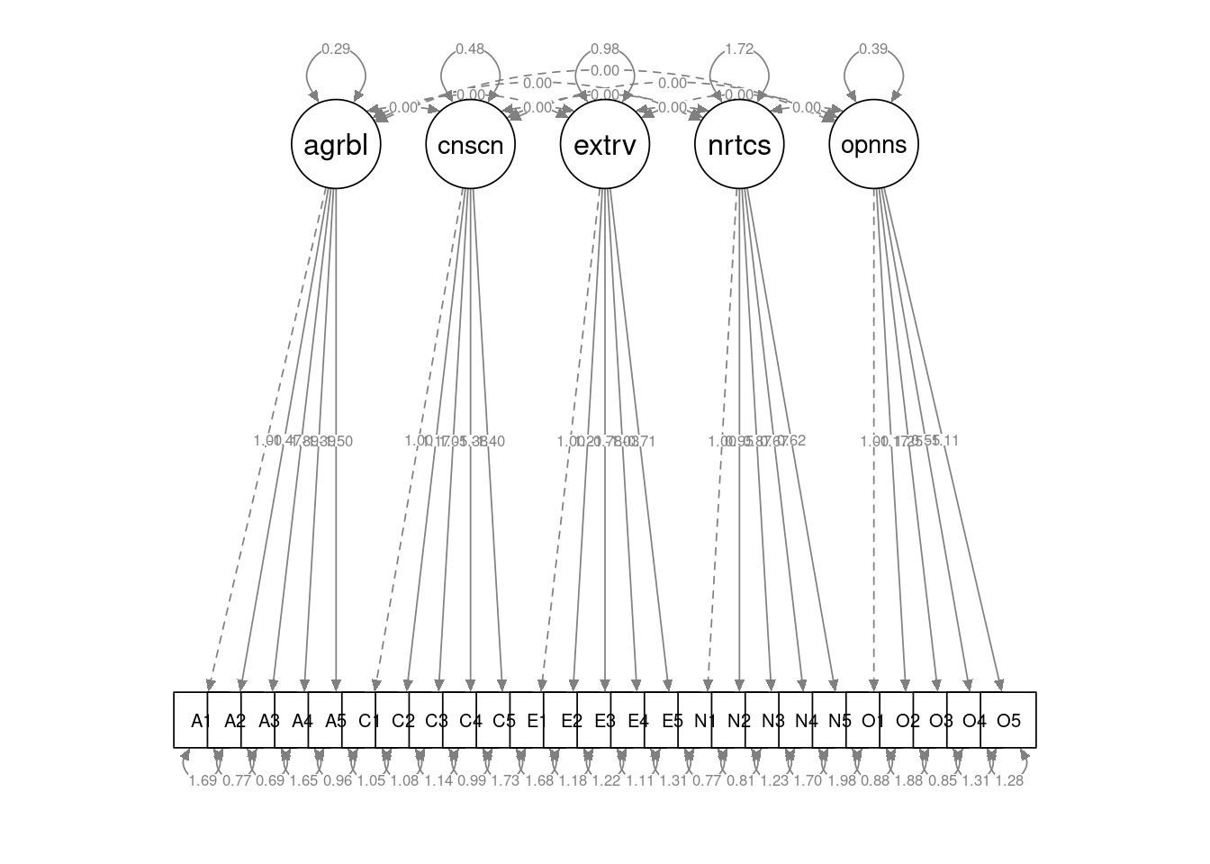
11.6 General SEM models
General SEM models can be estimated with the lavaan:sem() function. As in the lavaan::cfa() function, this allows you to specify latent variables via the =~ operator. You can also specify further path regressions, linking observed variables to other observed variables and/or to factors. As an example, we will analyse data from the speed dating experiment, which is available in the sdamr package as speeddate.
In this example, we will focus on ratings by participants on how physically attractive (date_attr), fun (date_fun), sincere (date_sinc), intelligent (date_intel), and ambitious (date_amb) they find them, as well as a rating of their overall liking of their date (date_like). The dating partner also provided the same ratings for the participants (same variables, but with other_ prepended).
In this first model, we will assume that more “frivolous” aspects of a potential partner (e.g. physical attractiveness and fun) are treated as distinct from more serious aspects of a potential partner (e.g., intelligence, ambition, and sincerity). This can be formalized in a SEM model by assuming different latent variables for each. By formulating these as latent variables, we can also determine the weight of each of the observed variables in determining the latent variables (via the factor loadings).
In the model below, we assume whether a person likes their date also depends on the reciprocal liking by their date of them. This is implemented by assuming that e.g. date_like is causally linked to the four latent variables d_frivolous, d_serious, o_frivolous, and o_serious. A similar assumption is made for other_like.
# load the data
data("speeddate", package="sdamr")

# specify the model
speed_mod_spec <- '
  # define latent variables
  d_frivolous =~ date_attr + date_fun
  d_serious =~ date_sinc + date_intel + date_amb

  o_frivolous =~ other_attr + other_fun
  o_serious =~ other_sinc + other_intel + other_amb

  # regressions
  date_like ~ d_frivolous + d_serious + o_frivolous + o_serious
  other_like ~ o_frivolous + o_serious + d_frivolous + d_serious
'

# estimate the model
speed_mod <- lavaan::sem(speed_mod_spec, data=speeddate)
The structural relations can be depicted with the code below. Note that we set various arguments in the semPlot::semPaths() function. To get a nice looking plot for your own data, it will pay to try different values of this. The semPaths() function is very flexible, but doesn’t generally provide the best looking plots by default. You should have a look at the help file to see all the possible options to make the plot look better (i.e. by typing ?semPlot::semPaths).
semPlot::semPaths(speed_mod, layout="tree2", sizeMan=7, residuals=TRUE, whatLabels = "est", nCharNodes = 12, normalize=TRUE, width=12, height=6)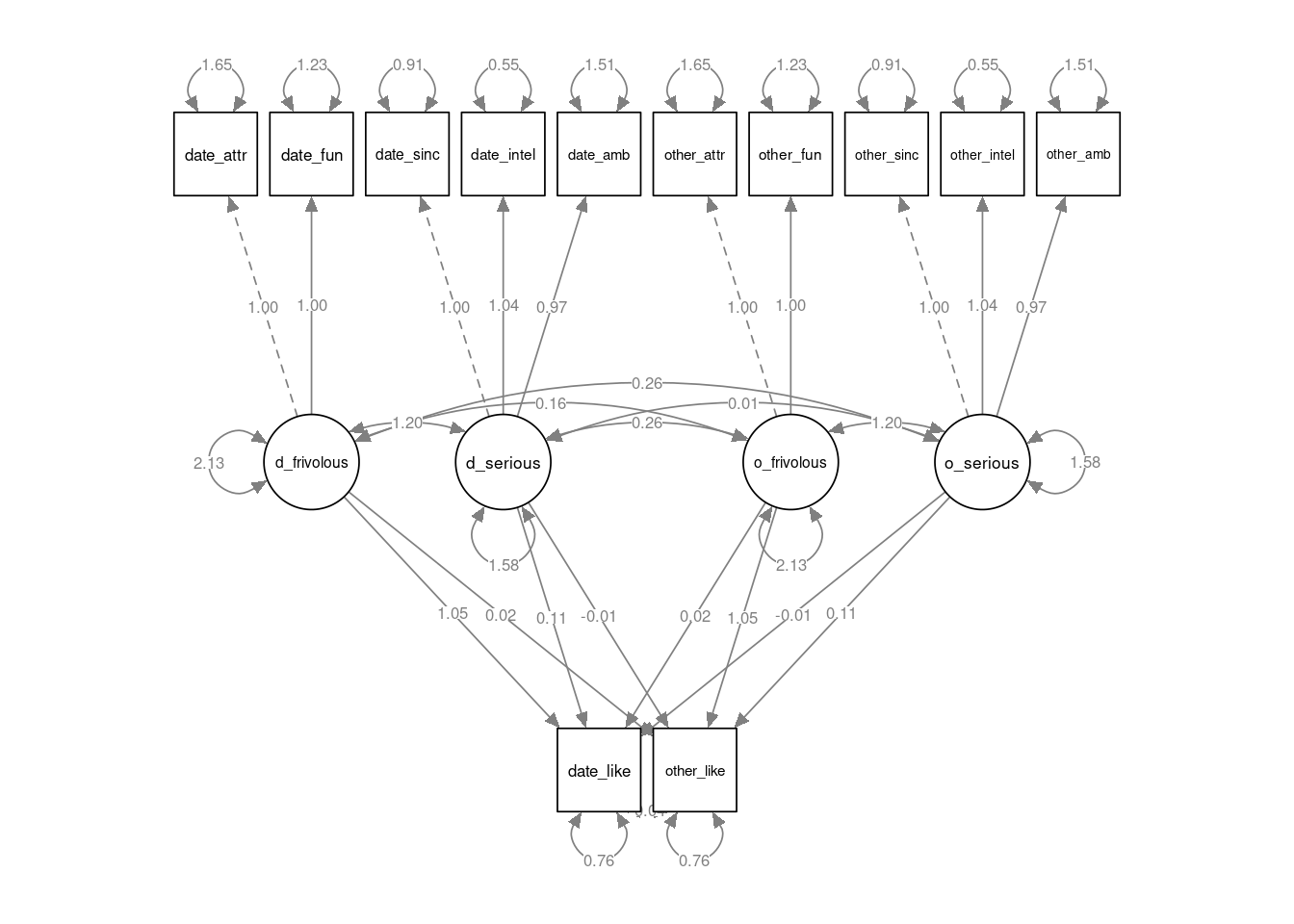
The parameter estimates and tests, as well as additional fit measures for the model, are obtained as:
## lavaan 0.6.16 ended normally after 46 iterations
##
##   Estimator                                         ML
##   Optimization method                           NLMINB
##   Number of model parameters                        37
##
##                                                   Used       Total
##   Number of observations                          1238        1562
##
## Model Test User Model:
##
##   Test statistic                               259.333
##   Degrees of freedom                                41
##   P-value (Chi-square)                           0.000
##
## Model Test Baseline Model:
##
##   Test statistic                              7562.059
##   Degrees of freedom                                66
##   P-value                                        0.000
##
## User Model versus Baseline Model:
##
##   Comparative Fit Index (CFI)                    0.971
##   Tucker-Lewis Index (TLI)                       0.953
##
## Loglikelihood and Information Criteria:
##
##   Loglikelihood user model (H0)             -25604.915
##   Loglikelihood unrestricted model (H1)     -25475.248
##
##   Akaike (AIC)                               51283.830
##   Bayesian (BIC)                             51473.316
##   Sample-size adjusted Bayesian (SABIC)      51355.788
##
## Root Mean Square Error of Approximation:
##
##   RMSEA                                          0.066
##   90 Percent confidence interval - lower         0.058
##   90 Percent confidence interval - upper         0.073
##   P-value H_0: RMSEA <= 0.050                    0.000
##   P-value H_0: RMSEA >= 0.080                    0.001
##
## Standardized Root Mean Square Residual:
##
##   SRMR                                           0.036
##
## Parameter Estimates:
##
##   Standard errors                             Standard
##   Information                                 Expected
##   Information saturated (h1) model          Structured
##
## Latent Variables:
##                    Estimate  Std.Err  z-value  P(>|z|)
##   d_frivolous =~
##     date_attr         1.000
##     date_fun          1.003    0.037   26.962    0.000
##   d_serious =~
##     date_sinc         1.000
##     date_intel        1.036    0.035   29.722    0.000
##     date_amb          0.972    0.039   24.959    0.000
##   o_frivolous =~
##     other_attr        1.000
##     other_fun         1.003    0.037   26.962    0.000
##   o_serious =~
##     other_sinc        1.000
##     other_intel       1.036    0.035   29.722    0.000
##     other_amb         0.972    0.039   24.959    0.000
##
## Regressions:
##                    Estimate  Std.Err  z-value  P(>|z|)
##   date_like ~
##     d_frivolous       1.051    0.059   17.933    0.000
##     d_serious         0.113    0.056    2.011    0.044
##     o_frivolous       0.019    0.045    0.433    0.665
##     o_serious        -0.008    0.051   -0.153    0.878
##   other_like ~
##     o_frivolous       1.051    0.059   17.933    0.000
##     o_serious         0.113    0.056    2.011    0.044
##     d_frivolous       0.019    0.045    0.433    0.665
##     d_serious        -0.008    0.051   -0.153    0.878
##
## Covariances:
##                    Estimate  Std.Err  z-value  P(>|z|)
##   d_frivolous ~~
##     d_serious         1.196    0.082   14.566    0.000
##     o_frivolous       0.156    0.081    1.934    0.053
##     o_serious         0.263    0.066    3.974    0.000
##   d_serious ~~
##     o_frivolous       0.263    0.066    3.974    0.000
##     o_serious         0.006    0.053    0.119    0.905
##   o_frivolous ~~
##     o_serious         1.196    0.082   14.566    0.000
##  .date_like ~~
##    .other_like       -0.038    0.044   -0.872    0.383
##
## Variances:
##                    Estimate  Std.Err  z-value  P(>|z|)
##    .date_attr         1.649    0.086   19.262    0.000
##    .date_fun          1.231    0.074   16.708    0.000
##    .date_sinc         0.914    0.053   17.385    0.000
##    .date_intel        0.546    0.045   12.258    0.000
##    .date_amb          1.510    0.072   20.869    0.000
##    .other_attr        1.649    0.086   19.262    0.000
##    .other_fun         1.231    0.074   16.708    0.000
##    .other_sinc        0.914    0.053   17.385    0.000
##    .other_intel       0.546    0.045   12.258    0.000
##    .other_amb         1.510    0.072   20.869    0.000
##    .date_like         0.765    0.070   10.928    0.000
##    .other_like        0.765    0.070   10.928    0.000
##     d_frivolous       2.132    0.147   14.494    0.000
##     d_serious         1.584    0.101   15.726    0.000
##     o_frivolous       2.132    0.147   14.494    0.000
##     o_serious         1.584    0.101   15.726    0.000
These results indicate that there is potentially little covariance between the latent variables for the participants (d_frivolous and d_serious) and for their dates (other_frivolous and other_serious). However, the “frivolous” and “serious” aspects of participants do appear correlated, and similarly for their dates.
These correlations can be captured by assuming residual covariances between factors are non-zero, but also by assuming a hierarchical factor structure, where a latent variable higher up in the structure determines the values of the latent variables below in the structure. The lavaan syntax allows you to specify such higher-order latent variables with the same =~ operator, by naming the higher-order latent variable on the left-hand side, and the latent variables that load onto this higher-order latent variable on the right-hand side. In the model below, we assume that it is these higher-order latent variables which “cause” the overall liking of each person by their dating partner (date_like and other_like).
speed_mod2_spec <- '
  # define latent variables
  d_frivolous =~ date_attr + date_fun
  d_serious =~ date_sinc + date_intel + date_amb
  d_overall =~ d_frivolous + d_serious

  o_frivolous =~ other_attr + other_fun
  o_serious =~ other_sinc + other_intel + other_amb
  o_overall =~ o_frivolous + o_serious

  # regressions
  date_like ~ d_overall
  other_like ~ o_overall

  # covariances
  date_like ~~ 0*other_like
'
speed_mod2 <- lavaan::sem(speed_mod2_spec, data=speeddate)
A plot of the model is obtained via:
semPlot::semPaths(speed_mod2, layout="tree2", sizeMan=7, residuals=TRUE, whatLabels = "est", nCharNodes = 12, normalize=TRUE, width=12, height=6)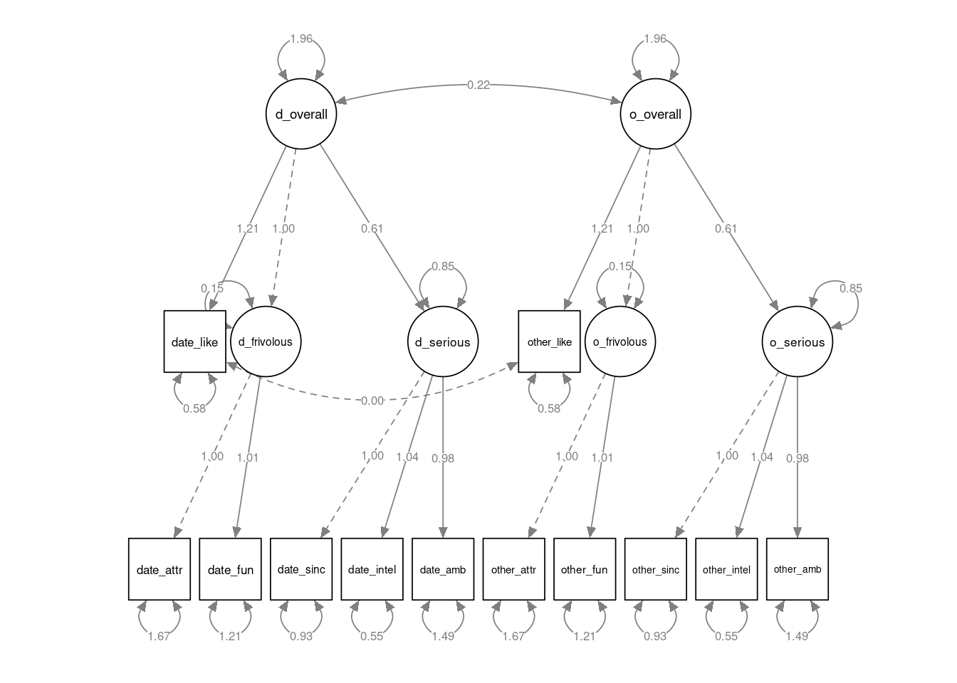
The parameter estimates and tests, as well as additional fit measures for the model, are obtained as:
## lavaan 0.6.16 ended normally after 38 iterations
##
##   Estimator                                         ML
##   Optimization method                           NLMINB
##   Number of model parameters                        29
##
##                                                   Used       Total
##   Number of observations                          1238        1562
##
## Model Test User Model:
##
##   Test statistic                               313.884
##   Degrees of freedom                                49
##   P-value (Chi-square)                           0.000
##
## Model Test Baseline Model:
##
##   Test statistic                              7562.059
##   Degrees of freedom                                66
##   P-value                                        0.000
##
## User Model versus Baseline Model:
##
##   Comparative Fit Index (CFI)                    0.965
##   Tucker-Lewis Index (TLI)                       0.952
##
## Loglikelihood and Information Criteria:
##
##   Loglikelihood user model (H0)             -25632.190
##   Loglikelihood unrestricted model (H1)     -25475.248
##
##   Akaike (AIC)                               51322.380
##   Bayesian (BIC)                             51470.897
##   Sample-size adjusted Bayesian (SABIC)      51378.780
##
## Root Mean Square Error of Approximation:
##
##   RMSEA                                          0.066
##   90 Percent confidence interval - lower         0.059
##   90 Percent confidence interval - upper         0.073
##   P-value H_0: RMSEA <= 0.050                    0.000
##   P-value H_0: RMSEA >= 0.080                    0.001
##
## Standardized Root Mean Square Residual:
##
##   SRMR                                           0.042
##
## Parameter Estimates:
##
##   Standard errors                             Standard
##   Information                                 Expected
##   Information saturated (h1) model          Structured
##
## Latent Variables:
##                    Estimate  Std.Err  z-value  P(>|z|)
##   d_frivolous =~
##     date_attr         1.000
##     date_fun          1.012    0.038   26.873    0.000
##   d_serious =~
##     date_sinc         1.000
##     date_intel        1.039    0.035   29.354    0.000
##     date_amb          0.981    0.039   24.979    0.000
##   d_overall =~
##     d_frivolous       1.000
##     d_serious         0.608    0.033   18.604    0.000
##   o_frivolous =~
##     other_attr        1.000
##     other_fun         1.012    0.038   26.873    0.000
##   o_serious =~
##     other_sinc        1.000
##     other_intel       1.039    0.035   29.354    0.000
##     other_amb         0.981    0.039   24.979    0.000
##   o_overall =~
##     o_frivolous       1.000
##     o_serious         0.608    0.033   18.604    0.000
##
## Regressions:
##                    Estimate  Std.Err  z-value  P(>|z|)
##   date_like ~
##     d_overall         1.206    0.051   23.817    0.000
##   other_like ~
##     o_overall         1.206    0.051   23.817    0.000
##
## Covariances:
##                    Estimate  Std.Err  z-value  P(>|z|)
##  .date_like ~~
##    .other_like        0.000
##   d_overall ~~
##     o_overall         0.215    0.064    3.370    0.001
##
## Variances:
##                    Estimate  Std.Err  z-value  P(>|z|)
##    .date_attr         1.667    0.086   19.368    0.000
##    .date_fun          1.213    0.074   16.455    0.000
##    .date_sinc         0.925    0.053   17.373    0.000
##    .date_intel        0.548    0.045   12.098    0.000
##    .date_amb          1.494    0.072   20.692    0.000
##    .other_attr        1.667    0.086   19.368    0.000
##    .other_fun         1.213    0.074   16.455    0.000
##    .other_sinc        0.925    0.053   17.373    0.000
##    .other_intel       0.548    0.045   12.098    0.000
##    .other_amb         1.494    0.072   20.692    0.000
##    .date_like         0.576    0.086    6.693    0.000
##    .other_like        0.576    0.086    6.693    0.000
##    .d_frivolous       0.155    0.073    2.125    0.034
##    .d_serious         0.849    0.062   13.732    0.000
##     d_overall         1.960    0.149   13.185    0.000
##    .o_frivolous       0.155    0.073    2.125    0.034
##    .o_serious         0.849    0.062   13.732    0.000
##     o_overall         1.960    0.149   13.185    0.000
11.7 Exploratory factor analysis with the psych package
We will just cover the very basics of Exploratory Factor Analysis (EFA) here. In EFA, each “factor” (which is a latent variable in the model) is related to all observed variables (sometimes also called the “manifest” variables).
EFA is implemented in the factanal() function from the stats package (base R), and the fa() function in the psych package. We will focus on the latter function here. The psych package comes with various additional tools useful for EFA, and adheres to the conventions for EFA in psychology.
11.7.1 Determining the number of factors with Parallel Analysis
A first useful function implements so-called “parallel analysis” to determine the optimal number of underlying factors for a given set of observed variables. This method, whilst somewhat “hacky”, tends to work reasonably well in practice.
Parallel analysis (see e.g. Hayton, Allen, and Scarpello 2004) focuses on the common variance “explained” by each factor. It uses so-called eigenvalues as the measure of common variance accounted for by the factors. An eigenvalue larger than 1 indicates that a factor accounts for more variance than that of a single variable (i.e. it accounts for shared variation between the variables). However, eigenvalues can be larger than 1 due to sampling error, even though a factor in reality does not account for substantial shared variation. Parallel analysis aims to compare the eigenvalues for factors to those of random data (where there is no shared variation). According to parallel analysis, the optimal number of factors is the number of factors that have larger eigenvalues than would be obtained for random data.
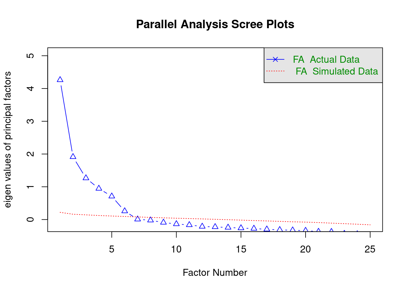
A parallel analysis can be conducted via the fa.parallel() function from the psych() package. The first argument to this function, called x, can be either a data.frame containing just the variables you want to include in the EFA, or a correlation matrix. In a second argument, called fa, you can specify that you want to use EFA (fa="fa"), a principal components analysis (fa="pc"), or both (fa="both"). Here, we will just ask for a factor analysis. On the first line of the code below, we first exclude the last three columns (gender, education, and age) from the data, and then ask for a parallel analysis:
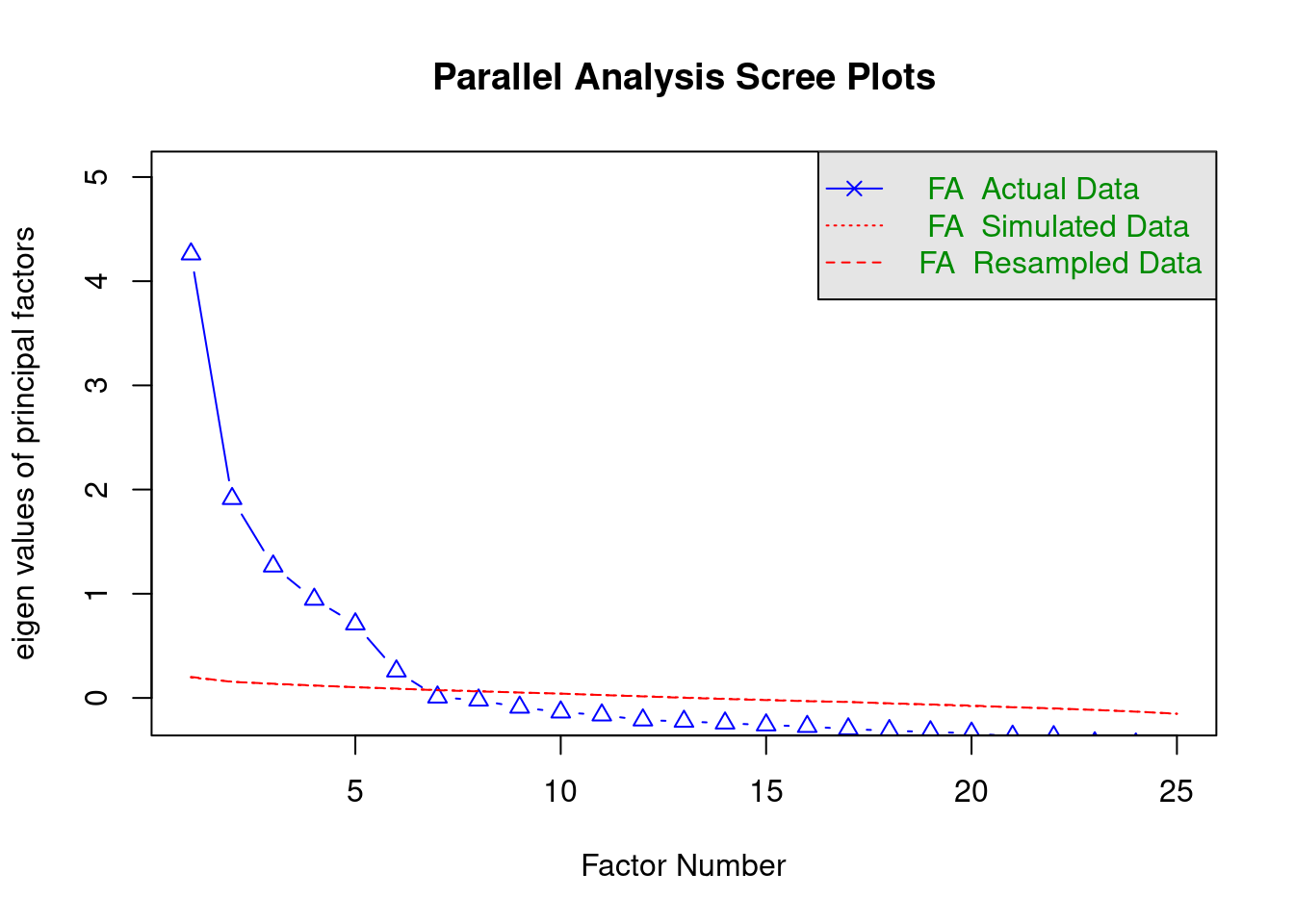
## Parallel analysis suggests that the number of factors = 6 and the number of components = NAThe plot shows the eigenvalues for the different factors (ordered in magnitude) as blue triangles, and eigenvalues for random data as red lines. There is also a message indicating the optimal number of factors according to the analysis, which is 6, as there are six blue triangles above the red line.
We could obtain the same result via a correlation matrix, which can be computed with the cor() function. Note that if there are missing values in the data, by default this would return a missing value in the correlation matrix. We can avoid this by explicitly stating how we want to deal with missing variables (in this case, for each pair of variables, use the complete cases).
# compute correlation matrix from pairwise complete cases
bfi_cor <- cor(bfi[,-c(26:28)], use="pairwise.complete.obs")
If you use a correlation matrix, you should also specify the number of observations used to compute the correlation. A lower bound on this can be computed via the complete.cases() function, which returns a logical vector with each element equaling TRUE when all variables in a row of the data are not missing. By summing up these logical values (TRUE has value 1, and FALSE value 0), you get the number of complete cases.
We can now finally perform the analysis:
## Parallel analysis suggests that the number of factors = 6 and the number of components = NANote that there is nothing to be gained from using a correlation matrix rather than the “raw” data. However, it is instructive to see that EFA only needs a correlation matrix.
11.7.2 Estimating and rotating EFA solutions
EFA can be performed via the fa() function from the psych package. Like the psych::fa.parallel() function, the first argument, now called r, can be a data.frame or a correlation or covariance matrix. The second argument, called nfactors, is used to set how many factors you want to include in the model. A further argument, called rotate, is used to set the rotation method. By default, this is Oblimin rotation, a form of oblique rotation. There are many other options (see the help file ?psych::fa), including "none" (no rotation), "varimax" (a popular form of orthogonal rotation), and "promax" (a popular form of oblique rotation). The argument fm is used to specify the estimation method, for which we will use fm="ml" to obtain maximum likelihood estimation.
Here is an example without rotation:
## Factor Analysis using method =  ml
## Call: psych::fa(r = bfi[, -c(26:28)], nfactors = 6, rotate = "none",
##     fm = "ml")
## Standardized loadings (pattern matrix) based upon correlation matrix
##      ML1   ML2   ML3   ML4   ML5   ML6   h2   u2 com
## A1  0.24 -0.03  0.09  0.01 -0.37  0.36 0.33 0.67 2.9
## A2 -0.40  0.35 -0.11  0.10  0.38 -0.21 0.50 0.50 3.8
## A3 -0.46  0.39 -0.19  0.09  0.31 -0.06 0.51 0.49 3.3
## A4 -0.37  0.20 -0.04  0.25  0.21  0.02 0.28 0.72 3.1
## A5 -0.54  0.29 -0.23  0.05  0.20  0.08 0.48 0.52 2.4
## C1 -0.28  0.18  0.46  0.03  0.00  0.16 0.35 0.65 2.3
## C2 -0.27  0.25  0.53  0.17  0.08  0.22 0.50 0.50 2.8
## C3 -0.27  0.13  0.39  0.23  0.07  0.05 0.31 0.69 2.9
## C4  0.45 -0.01 -0.52 -0.16  0.06  0.23 0.55 0.45 2.6
## C5  0.49  0.01 -0.34 -0.24  0.12  0.05 0.43 0.57 2.5
## E1  0.36 -0.30  0.26  0.05  0.27  0.15 0.39 0.61 4.2
## E2  0.58 -0.22  0.22 -0.02  0.33  0.09 0.55 0.45 2.3
## E3 -0.46  0.43 -0.15 -0.18 -0.05  0.18 0.48 0.52 2.9
## E4 -0.54  0.33 -0.29  0.15 -0.15  0.15 0.56 0.44 2.9
## E5 -0.42  0.42  0.11 -0.04 -0.20 -0.02 0.40 0.60 2.6
## N1  0.59  0.56  0.04  0.08 -0.17 -0.08 0.71 0.29 2.2
## N2  0.58  0.56  0.08  0.03 -0.13 -0.14 0.69 0.31 2.3
## N3  0.52  0.49  0.02  0.01  0.08  0.05 0.52 0.48 2.1
## N4  0.58  0.23  0.04 -0.10  0.27  0.08 0.48 0.52 1.9
## N5  0.41  0.31 -0.01  0.15  0.22  0.10 0.34 0.66 2.9
## O1 -0.28  0.24  0.14 -0.41 -0.01  0.15 0.34 0.66 3.1
## O2  0.20  0.05 -0.25  0.39  0.05  0.18 0.29 0.71 2.9
## O3 -0.34  0.33  0.09 -0.49  0.01  0.11 0.48 0.52 2.9
## O4  0.10  0.18  0.14 -0.31  0.30  0.05 0.25 0.75 3.4
## O5  0.19 -0.06 -0.22  0.47 -0.05  0.24 0.37 0.63 2.5
##
##                        ML1  ML2  ML3  ML4  ML5  ML6
## SS loadings           4.40 2.35 1.54 1.22 0.99 0.57
## Proportion Var        0.18 0.09 0.06 0.05 0.04 0.02
## Cumulative Var        0.18 0.27 0.33 0.38 0.42 0.44
## Proportion Explained  0.40 0.21 0.14 0.11 0.09 0.05
## Cumulative Proportion 0.40 0.61 0.75 0.86 0.95 1.00
##
## Mean item complexity =  2.8
## Test of the hypothesis that 6 factors are sufficient.
##
## df null model =  300  with the objective function =  7.23 with Chi Square =  20163.79
## df of  the model are 165  and the objective function was  0.36
##
## The root mean square of the residuals (RMSR) is  0.02
## The df corrected root mean square of the residuals is  0.03
##
## The harmonic n.obs is  2762 with the empirical chi square  661.28  with prob <  1.4e-60
## The total n.obs was  2800  with Likelihood Chi Square =  1013.79  with prob <  4.6e-122
##
## Tucker Lewis Index of factoring reliability =  0.922
## RMSEA index =  0.043  and the 90 % confidence intervals are  0.04 0.045
## BIC =  -295.88
## Fit based upon off diagonal values = 0.99
## Measures of factor score adequacy
##                                                    ML1  ML2  ML3  ML4  ML5  ML6
## Correlation of (regression) scores with factors   0.95 0.92 0.86 0.82 0.81 0.71
## Multiple R square of scores with factors          0.90 0.84 0.74 0.67 0.65 0.51
## Minimum correlation of possible factor scores     0.81 0.68 0.48 0.34 0.30 0.02
The output is rather extensive. A key table is the first one, with standardized factor loadings in the columns labelled ML.
You can just check the factor loadings via the stat::loadings() function. This allows you to not print loadings below a certain value (e.g. .10), by setting the cutoff argument. Below we will show the loadings obtained after Varimax rotation:
bfi_fa <- psych::fa(bfi[,-c(26:28)], nfactors = 6, rotate="varimax", fm="ml")
loadings(bfi_fa, cutoff=.1)
##
## Loadings:
## ML2 ML1 ML3 ML5 ML4 ML6
## A1 0.110 -0.526 -0.119 0.153
## A2 0.233 0.135 0.646
## A3 0.361 0.118 0.590 0.134
## A4 0.208 0.243 0.386 -0.127
## A5 -0.136 0.435 0.109 0.456 0.220
## C1 0.549 0.170
## C2 0.677 0.158
## C3 0.541 0.115
## C4 0.227 -0.608 -0.113 -0.149 0.308
## C5 0.282 -0.177 -0.534 0.159
## E1 -0.584 -0.114 0.145
## E2 0.236 -0.677 -0.104 0.134
## E3 0.570 0.102 0.174 0.222 0.248
## E4 -0.126 0.669 0.114 0.212 -0.126 0.143
## E5 0.503 0.306 0.198
## N1 0.807 -0.164 -0.128
## N2 0.803 -0.126 -0.166
## N3 0.711
## N4 0.555 -0.331 -0.154 0.181
## N5 0.513 -0.156 -0.160 0.156
## O1 0.243 0.137 0.467 0.217
## O2 0.163 -0.485 0.142
## O3 0.333 0.102 0.556 0.223
## O4 0.213 -0.159 0.129 0.348 0.207
## O5 -0.583 0.132
##
## ML2 ML1 ML3 ML5 ML4 ML6
## SS loadings 2.698 2.623 2.010 1.618 1.462 0.661
## Proportion Var 0.108 0.105 0.080 0.065 0.058 0.026
## Cumulative Var 0.108 0.213 0.293 0.358 0.416 0.443Note that the factors are ordered according to how much variance they explain. In this case, the second factor ML2 accounts for the most variance. A different solution is obtained with Promax rotation:
## Loading required namespace: GPArotation##
## Loadings:
## ML1 ML2 ML3 ML5 ML4 ML6
## A1 0.103 0.119 -0.616 0.149 0.152
## A2 0.147 0.103 0.645
## A3 0.274 0.525 0.141
## A4 0.113 0.202 0.322 0.174
## A5 0.346 -0.148 0.337 0.237
## C1 0.590 -0.109 -0.107
## C2 -0.108 0.748
## C3 0.590 -0.105
## C4 -0.631 -0.132 0.143 0.417
## C5 0.141 -0.539 0.274
## E1 -0.678 -0.127 0.196
## E2 -0.733 0.112
## E3 0.547 -0.145 0.342
## E4 0.669 0.197 0.142
## E5 0.510 0.179 0.229 -0.150
## N1 0.232 0.902 -0.112
## N2 0.186 0.911 -0.142
## N3 0.686 0.122
## N4 -0.308 0.428 0.232
## N5 -0.140 0.440 0.176 0.137
## O1 0.191 -0.110 -0.413 0.343
## O2 0.100 0.504
## O3 0.288 -0.499 0.382
## O4 -0.224 0.104 0.121 -0.330 0.301
## O5 -0.121 0.603
##
## ML1 ML2 ML3 ML5 ML4 ML6
## SS loadings 2.647 2.636 2.115 1.403 1.365 1.004
## Proportion Var 0.106 0.105 0.085 0.056 0.055 0.040
## Cumulative Var 0.106 0.211 0.296 0.352 0.407 0.447